This is part 4 of the Math Foundations series.
The previous post introduced the key probability distributions. This one answers a deeper question: what happens when you repeatedly take samples and compute statistics from them? The answer turns out to be surprisingly universal, and it’s the reason the normal distribution shows up everywhere.
Sampling Distributions
Suppose you want to know the average height of adults in a country. You can’t measure everyone, so you take a sample of $n$ people and compute the sample mean $\bar{x}$. That number is an estimate - a different sample of $n$ people would give a slightly different $\bar{x}$.
Now imagine repeating this: draw a sample, compute $\bar{x}$, write it down. Draw another sample, compute $\bar{x}$, write it down. Do this thousands of times. The collection of all those $\bar{x}$ values forms a distribution - the sampling distribution of the mean.
This isn’t a theoretical curiosity. Every time you compute a statistic from data, that statistic has a sampling distribution. Understanding it tells you:
- How much your estimate might vary from sample to sample
- How confident you can be in your result
- Whether an observed difference is real or just noise
Three key facts about the sampling distribution of $\bar{X}$:
- Centre: it’s centred at the true population mean $\mu$. Your sample means aren’t systematically too high or too low.
- Spread: it gets narrower as $n$ increases. Larger samples give more consistent estimates.
- Shape: regardless of the population’s shape, the sampling distribution becomes normal for large enough $n$. This is the Central Limit Theorem.
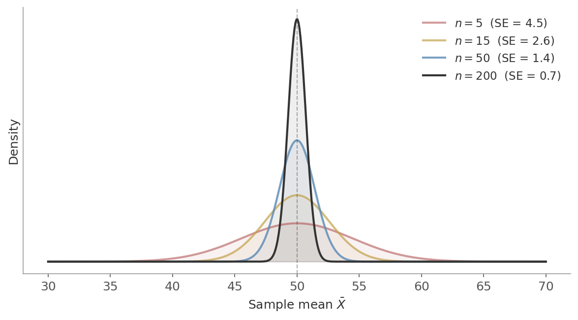 Figure 1: The sampling distribution of $\bar{X}$ for different sample sizes. All four are centred at $\mu = 50$, but larger samples produce tighter distributions. At $n = 200$, the spread is just 0.7.
Law of Large Numbers
Before the CLT, one simpler result that builds the intuition.
As the sample size grows, the sample mean converges to the population mean:
$$\bar{X}_n \xrightarrow{p} \mu \quad \text{as } n \to \infty$$This is the formal version of “flip a coin enough times and you’ll get close to 50% heads.” The LLN doesn’t say anything about the distribution of the sample mean - just that it gets closer to $\mu$.
import numpy as np

np.random.seed(42)
# Simulate coin flips - running average converges to 0.5
flips = np.random.binomial(1, 0.5, size=10000)
running_mean = np.cumsum(flips) / np.arange(1, 10001)

print(f"After    10 flips: mean = {running_mean[9]:.3f}")
print(f"After   100 flips: mean = {running_mean[99]:.3f}")
print(f"After  1000 flips: mean = {running_mean[999]:.3f}")
print(f"After 10000 flips: mean = {running_mean[9999]:.3f}")

# After    10 flips: mean = 0.600
# After   100 flips: mean = 0.470
# After  1000 flips: mean = 0.497
# After 10000 flips: mean = 0.492
The wobble shrinks. That’s the LLN in action.
The LLN does not say that future results will “balance out” past ones. If you flip 10 heads in a row, the probability of the next flip being heads is still 50%. The convergence happens because the 10 early heads get diluted by thousands of future flips - not because the coin “remembers” it owes you tails. This misconception is called the gambler’s fallacy.
The Central Limit Theorem
This is the main result.
Take any distribution with finite mean $\mu$ and variance $\sigma^2$. Draw $n$ independent values and compute their mean $\bar{X}$. As $n$ grows:
$$\bar{X} \xrightarrow{d} \mathcal{N}\left(\mu, \frac{\sigma^2}{n}\right)$$The distribution of the sample mean approaches a normal distribution - regardless of the original distribution.
Read that again. The original distribution can be uniform, exponential, binomial, wildly skewed - it doesn’t matter. Average enough independent values and the distribution of that average becomes normal.
This is why:
- Confidence intervals use the normal distribution - the CLT says the sample mean is normally distributed, so you can build intervals around it.
- Hypothesis tests assume normality of the test statistic - most test statistics are means or functions of means, and the CLT is what justifies treating them as normal.
- The normal distribution appears everywhere - many real-world quantities (heights, measurement errors, stock returns) are sums of many small, independent effects, and the CLT says any such sum trends toward normal.
Seeing It
The best way to understand the CLT is to watch it happen. Take the $\text{Exponential}(1)$ distribution - heavily right-skewed, with most values near zero and a long tail to the right. Now repeatedly draw $n$ values and compute their mean. Each panel below shows the distribution of 50,000 such sample means:
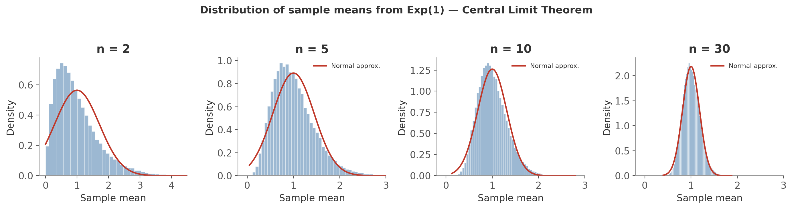 Figure 2: The CLT in action with $\text{Exponential}(1)$ ($\mu = 1$, $\sigma = 1$). Each panel shows the distribution of 50,000 sample means for a given $n$. The red curve is the normal approximation $\mathcal{N}(\mu, \sigma^2/n)$.
- $n = 2$: averaging just two values already reduces the skew noticeably compared to the raw exponential. The peak has moved toward the mean and the tail is shorter.
- $n = 5$: the histogram is roughly bell-shaped. The red normal curve is a decent fit, though slight skew remains.
- $n = 10$: the normal approximation is now a good fit. Most of the skew is gone.
- $n = 30$: the histogram and the normal curve are nearly indistinguishable. The distribution has also gotten much narrower - the spread is $\sigma/\sqrt{30} \approx 0.18$, compared to $\sigma = 1$ for the raw distribution.
The original distribution was about as non-normal as it gets. Yet by $n = 30$, the sample means are normal and tightly concentrated around $\mu$. The CLT captures both facts - the normal shape and the narrowing - in one statement:
$$\bar{X} \approx \mathcal{N}\left(\mu, \frac{\sigma^2}{n}\right)$$The shape is normal. And the variance is $\sigma^2/n$ - it shrinks with sample size.
Standard Error
That $\sigma^2/n$ term is doing the practical work. Its square root has a name - the standard error:
The standard deviation of the sampling distribution of $\bar{X}$.
The SE is what makes the CLT practical. Once you know the sampling distribution is normal with standard deviation $SE$, you can make precise probability statements. For instance, 95% of sample means fall within $\pm 1.96 \times SE$ of $\mu$ - because that’s how the normal distribution works. That’s exactly where confidence intervals come from.
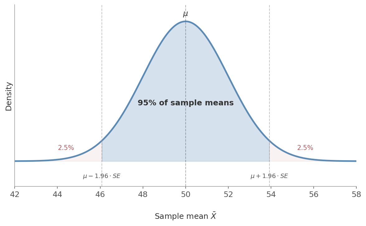 Figure 3: The sampling distribution of $\bar{X}$. The CLT gives the normal shape; the SE gives the width. Together they define the 95% interval: $\mu \pm 1.96 \times SE$. Only 2.5% of sample means land in each tail.
Double your sample size and the standard error shrinks to $\frac{1}{\sqrt{2}} \approx 71\%$ of its previous value. To halve the standard error, you need to quadruple the sample size. This square-root relationship is why there are diminishing returns to collecting more data.
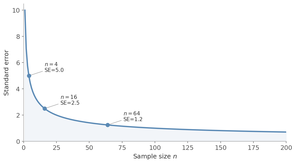 Figure 4: The $1/\sqrt{n}$ decay. Quadrupling the sample size from 4 to 16 halves the SE from 5.0 to 2.5. Quadrupling again to 64 halves it again to 1.2. Each doubling of precision costs four times the data.
A website has an average session duration of $\mu = 4.2$ minutes with $\sigma = 2.8$ minutes. You take a sample of $n = 100$ sessions.
$$SE = \frac{2.8}{\sqrt{100}} = 0.28 \text{ minutes}$$By the CLT, the sampling distribution of $\bar{X}$ is approximately $\mathcal{N}(4.2, 0.28^2)$. About 95% of sample means will fall within $\pm 2 \times 0.28 = \pm 0.56$ minutes of the true mean. If you increase to $n = 400$:
$$SE = \frac{2.8}{\sqrt{400}} = 0.14 \text{ minutes}$$Four times the data, half the standard error.
In practice, you rarely know $\sigma$ (the true population standard deviation). You estimate it from your data using $s$ (the sample standard deviation). When using the estimated $SE = \frac{s}{\sqrt{n}}$, the sampling distribution follows a t-distribution rather than a normal - which is why we introduced the t-distribution in the previous post.
How Large is “Large Enough”?
The rule of thumb is $n \geq 30$. But it depends on how non-normal the original distribution is:
- Symmetric distributions (uniform, triangular): $n = 5\text{-}10$ is often enough
- Moderately skewed: $n = 30$ works well
- Heavily skewed (exponential, Pareto): might need $n = 50\text{-}100$
The more skewed or heavy-tailed the original distribution, the larger your sample needs to be before the CLT kicks in.
Why This Matters
The CLT is the engine behind most of classical statistics:
- Confidence intervals: the normal shape + the SE give you $\bar{x} \pm z^* \cdot \frac{s}{\sqrt{n}}$. To see what “95% confidence” actually means, imagine this: a population has true mean $\mu = 100$. You draw a sample of $n = 25$ people, compute the sample mean and SE, and build an interval $\bar{x} \pm 1.96 \times SE$. That’s one confidence interval. Now do it again with a fresh sample of 25 - you get a different $\bar{x}$, a different interval. Repeat this 50 times. Each of the 50 intervals is centred at a different $\bar{x}$, but about 47-48 of them will contain the true $\mu$.
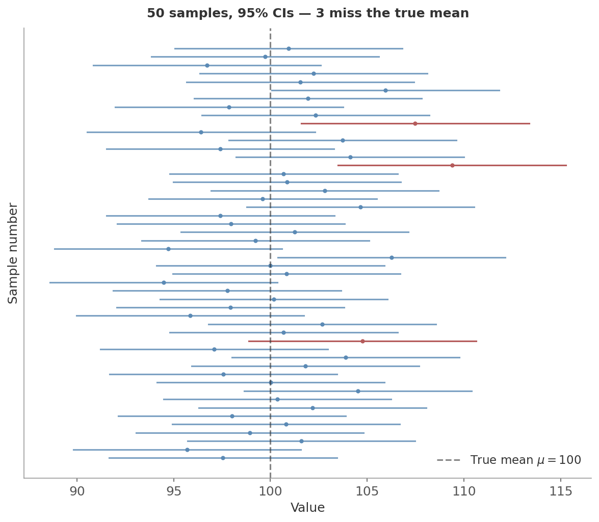 Figure 5: Each horizontal line is one confidence interval from one sample. The dot is that sample’s $\bar{x}$; the line extends $\pm 1.96 \times SE$ around it. The dashed vertical line is the true $\mu$. Blue intervals contain it; red ones miss. “95% confidence” means this procedure captures the true parameter about 95% of the time.
Hypothesis testing: under the null hypothesis, your test statistic (typically a mean or difference of means) has a known sampling distribution. The CLT is what lets you compute the probability of seeing a result as extreme as yours - the p-value.
A/B testing: the difference in conversion rates between two groups is a difference of means. With enough users, the CLT guarantees this difference is approximately normal - which is what lets you decide whether the difference is real or noise.
Model training: many loss functions involve averages over data points. The CLT is why gradient estimates from mini-batches work.
We’ll put all of this to work in the next post.
Next up: Hypothesis Testing & Confidence Intervals - how to decide if a difference is real or just noise.