This is part 2 of the ML Fundamentals series.
Linear regression gives you coefficients. But more features don’t always help - at some point the model starts fitting noise instead of signal. This post covers two connected problems: how to prevent overfitting (regularization) and how to choose which features to keep (feature selection).
The Bias-Variance Trade-off
Every predictive model makes two kinds of errors.
Bias: systematic error from wrong assumptions. A linear model fit to a quadratic relationship will consistently miss the curve - it underfits. No matter how much data you throw at it, the error from the wrong functional form stays.
Variance: sensitivity to the training data. A model with too many parameters can memorize the noise in one particular dataset, then fail on a new one - it overfits. The predictions change a lot depending on which training set you happened to draw.
The first two terms are under your control. The third is not - it’s the randomness inherent in the data.
Simple models (few parameters, strong assumptions) have high bias and low variance - they miss patterns but are stable. Complex models (many parameters, few assumptions) have low bias and high variance - they capture patterns but also capture noise. You can see this in learning curves.
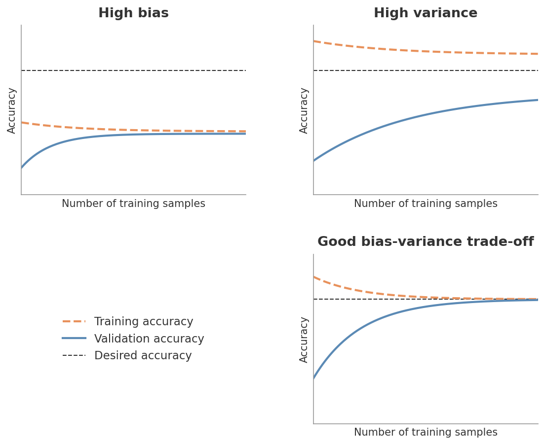 Figure 1: Learning curves under different bias-variance regimes. The orange dashed line is training accuracy, the blue solid line is validation accuracy, and the black dashed line is the desired accuracy. High bias (top-left): both curves plateau well below the target - more data won’t help. High variance (top-right): training accuracy is high but validation accuracy lags far behind - the model memorizes rather than generalizes. Good trade-off (bottom-right): both curves converge near the desired accuracy as training size grows.
The goal is to find the sweet spot where total error is minimized. Regularization is the main tool for doing this - it explicitly controls model complexity by penalizing large coefficients.
In practice, you don’t compute bias and variance separately. You observe their effects through the gap between training and validation performance. A large gap (low training error, high validation error) signals high variance. Uniformly high error on both signals high bias.
Regularization
The idea is straightforward: add a penalty term to the cost function that discourages large coefficients. This forces the model to find a solution that fits the data reasonably well and keeps the coefficients small. The result is a model that generalizes better to new data.
Ridge (L2)
The first term is the ordinary MSE. The second term penalizes the sum of squared coefficients. The parameter $\lambda$ controls the penalty strength.
Ridge shrinks all coefficients toward zero, but none of them reach it exactly. Every feature stays in the model - just with a smaller effect. This works well when you believe most features contribute something, and the problem is that the model is overweighting them.
The intercept $\beta_0$ is not penalized. It would make no sense to shrink the baseline prediction.
Lasso (L1)
Same structure, but the penalty uses the sum of absolute coefficient values instead of squared values.
The key difference: some coefficients are driven to exactly zero. Lasso doesn’t just shrink - it performs feature selection as part of the optimization. At a given $\lambda$, only the features that carry enough signal to justify their presence survive. The rest are removed entirely.
Why L1 Produces Zeros and L2 Doesn’t
This is one of those results that’s worth understanding rather than memorizing. There are two complementary explanations.
The gradient argument. The L2 penalty is $\beta^2$, which has gradient $2\beta$. As $\beta$ approaches zero, the gradient shrinks too - the penalty pushes toward zero with decreasing force. It asymptotically approaches but never arrives. The L1 penalty is $|\beta|$, which has a constant gradient of $\pm 1$ regardless of how close $\beta$ is to zero. The push toward zero never weakens. Once the penalty’s constant force exceeds the data’s pull away from zero, the coefficient snaps to exactly zero.
The geometric argument. Picture the MSE contours as ellipses in coefficient space, centered at the OLS solution. The constraint region for L2 is a circle (smooth, no corners). For L1 it’s a diamond (corners sitting on the axes, where one or more coefficients equal zero). As the ellipses expand from the OLS solution, they hit the L2 circle at a smooth point - almost certainly not on an axis. But they tend to hit the L1 diamond at a corner, which is exactly where coefficients are zero.
Elastic Net
The mixing parameter $\alpha$ controls the balance: $\alpha = 1$ is pure Lasso, $\alpha = 0$ is pure Ridge.
Elastic Net exists because Lasso has a weakness with correlated features. When two features are highly correlated, Lasso tends to pick one and zero out the other arbitrarily. The Ridge component in Elastic Net encourages correlated features to share the coefficient weight rather than fighting over it.
| Method | Penalty | Coefficients | Feature selection | Best for |
|---|---|---|---|---|
| Ridge (L2) | $\lambda \sum \beta_j^2$ | All shrink toward zero | No | Many small effects |
| Lasso (L1) | $\lambda \sum | \beta_j | $ | Some hit exactly zero |
| Elastic Net | Both | Mix of both behaviors | Yes | Correlated features |
Choosing Lambda and Scaling
The regularization parameter $\lambda$ controls the penalty strength. At $\lambda = 0$, you get plain OLS. As $\lambda$ increases, coefficients shrink further. Too much and the model underfits.
Cross-validation is the standard way to choose $\lambda$. Fit the model for a range of values (scikit-learn’s RidgeCV and LassoCV do this automatically), evaluate each on held-out folds, and pick the $\lambda$ with the best validation performance.
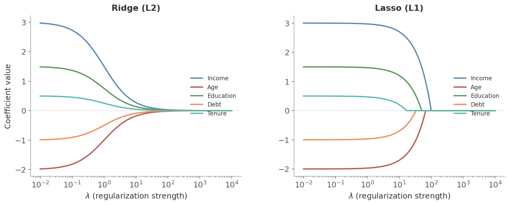 Figure 2: Coefficient paths as $\lambda$ increases. Left: Ridge shrinks all coefficients smoothly toward zero. Right: Lasso drives coefficients to exactly zero at different $\lambda$ values - the weaker signals vanish first, leaving only the strongest features.
The penalty treats all coefficients equally. If one feature is measured in dollars and another in percentages, their coefficients are on different scales - and the penalty hits them unevenly. A feature with naturally large values will have a small coefficient that gets penalized less, while a feature with small values will have a large coefficient that gets penalized more. Standardizing (zero mean, unit variance) puts all features on equal footing so the penalty is applied fairly.
Feature Selection
Regularization is one way to decide which features matter. But there’s a broader toolkit. Feature selection methods fall into three categories - filter, wrapper, and embedded - each trading computation time for selection quality.
Filter Methods
Filter methods evaluate features before training any model. They rank features by their statistical relationship with the target and discard the weak ones.
Correlation coefficients are the simplest filter. Pearson correlation measures linear relationships between a feature and the target. Spearman correlation captures monotonic relationships (including non-linear ones). A feature with near-zero correlation with the target probably isn’t useful.
Variance Inflation Factor (VIF) doesn’t measure feature-target relationships - it measures feature-feature relationships. VIF quantifies multicollinearity: how much a feature’s variance is inflated because it’s correlated with other features. A VIF above 5-10 means the feature is largely redundant with others in the model.
$$\text{VIF}_j = \frac{1}{1 - R_j^2}$$where $R_j^2$ is the R-squared from regressing feature $j$ on all other features. If the other features explain 90% of feature $j$’s variance, $\text{VIF}_j = 10$.
Mutual information captures any kind of statistical dependence - including non-linear relationships that correlation misses entirely. It measures how much knowing the value of a feature reduces uncertainty about the target. Zero mutual information means the feature and target are independent.
They’re model-agnostic and computationally cheap. But they evaluate each feature independently, so they miss interactions. Two features might be useless alone but informative together. Filters can’t see that.
Wrapper Methods
Wrapper methods train models with different feature subsets and evaluate their performance directly. They’re more expensive but can capture feature interactions.
Sequential Backward Selection (SBS)
Start with all features. Remove one at a time - specifically, the one whose removal hurts performance the least. Keep going until you reach the desired number of features.
Start with 5 features: {A, B, C, D, E}. Validation accuracy with all five: 0.82.
Round 1: Try removing each feature, train and evaluate:
- Remove A → 0.81
- Remove B → 0.80
- Remove C → 0.82
- Remove D → 0.78
- Remove E → 0.81
Removing C doesn’t hurt at all. Drop it. Remaining: {A, B, D, E}.
Round 2: Repeat with four features:
- Remove A → 0.80
- Remove B → 0.79
- Remove D → 0.76
- Remove E → 0.81
Removing E costs almost nothing. Drop it. Remaining: {A, B, D}.
Round 3: Now each removal hurts meaningfully. Stop here - {A, B, D} is the selected subset.
This is a greedy algorithm - it makes the locally best choice at each step, which doesn’t guarantee the globally optimal subset. But exhaustive search over all $2^p$ subsets is impractical for more than about 20 features.
Recursive Feature Elimination (RFE)
RFE is more principled than SBS because it uses the model’s own feature ranking. The process:
- Train the model on all features
- Rank features by importance (e.g. coefficient magnitude for linear models, impurity reduction for trees)
- Remove the lowest-ranked feature(s)
- Repeat until the desired number of features remains
The difference from SBS: instead of evaluating every possible removal, RFE asks the model which feature matters least and removes that one. This is faster and leverages the model’s internal knowledge about feature importance.
Embedded Methods
Embedded methods perform feature selection during training. The selection is built into the learning algorithm itself.
L1 Regularization (Lasso)
Already covered above. Lasso zeroes out irrelevant features as a natural part of the optimization. No separate selection step needed. This makes it the most natural embedded method for linear models.
Tree-Based Feature Importance
Decision trees and random forests provide a built-in measure of feature importance: how much each feature reduces impurity (Gini index or entropy) across all the splits where it’s used. Features that appear in many splits near the top of the tree are considered important.
It favors high-cardinality features (features with many unique values get more split opportunities) and handles correlated features poorly. When two features carry the same signal, the tree picks one and the other appears unimportant - even though they’re equally informative. Permutation importance is a more reliable alternative, though slower.
SHAP Values
The methods above tell you which features matter. SHAP goes further - it tells you how each feature affects each individual prediction, in both direction and magnitude.
SHAP (SHapley Additive exPlanations) is based on Shapley values from cooperative game theory. The idea: treat features as “players” cooperating to produce a prediction. The Shapley value fairly distributes the total “payout” (the difference between this prediction and the average prediction) among all features, accounting for interactions.
For a given prediction, the SHAP value of feature $j$ answers: “How much does feature $j$ contribute to the difference between this prediction and the average prediction?”
A positive SHAP value means the feature pushes the prediction higher. A negative value pushes it lower. The magnitude tells you how much. All SHAP values for one prediction sum to the difference between that prediction and the mean prediction.
SHAP is model-agnostic - it works with any model, not just trees or linear models. It handles feature interactions (the Shapley framework accounts for how features work together, not just individually). And it gives you per-prediction explanations, not just global rankings. The trade-off is computation time - exact SHAP is expensive ($O(2^p)$ for $p$ features). TreeSHAP is a fast exact algorithm for tree-based models. For other models, sampling-based approximations (KernelSHAP) are used.
A SHAP summary plot (beeswarm plot) gives you the global picture at a glance.
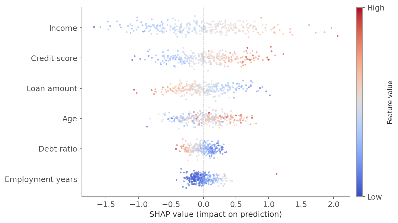 Figure 3: A SHAP beeswarm plot. Each row is a feature, sorted by importance (mean absolute SHAP value). Each dot is one observation - horizontal position shows how much that feature pushed the prediction above (right) or below (left) the average. Color indicates the feature’s value: red is high, blue is low. For “income,” red dots cluster on the right (high income pushes predictions up) and blue dots on the left (low income pushes predictions down).
Practical Notes
There’s no single right approach to feature selection. The right combination depends on the problem.
Start with filters to remove obvious noise - features with zero variance, near-zero correlation with the target, or extreme multicollinearity (high VIF). This is cheap and reduces the search space for more expensive methods.
Then use embedded or wrapper methods to refine. Lasso or Elastic Net for linear models. Tree-based importance or RFE for non-linear models. These account for feature interactions that filters miss.
When to use what:
- Few features (< 20): wrapper methods like RFE are feasible and thorough
- Many features (hundreds or more): filter methods first to prune, then L1 regularization
- Interpretability matters: SHAP - it gives you explanations, not just rankings
- Correlated features: Elastic Net or permutation importance rather than Lasso or tree-based importance
| Category | Method | Speed | Handles interactions | Handles correlation | Notes |
|---|---|---|---|---|---|
| Filter | Correlation | Fast | No | Detects it (VIF) | Good first pass |
| Filter | Mutual information | Fast | Pairwise only | No | Captures non-linear effects |
| Wrapper | SBS / RFE | Slow | Yes | Partially | Trains many models |
| Embedded | Lasso (L1) | Fast | No | Poorly (picks one) | Built into optimization |
| Embedded | Tree importance | Fast | Yes | Poorly (picks one) | Biased toward high cardinality |
| Model-agnostic | SHAP | Slow | Yes | Yes | Most informative, most expensive |
Next in the ML Fundamentals series: how to measure whether your model actually works - loss functions, metrics, and evaluation strategies.