This is part 3 of the Math Foundations series.
The previous post covered the rules of probability. This one is about what happens when you attach probability to outcomes - you get distributions. Distributions describe the shape of uncertainty: how likely each value is, where the mass concentrates, how the tails behave.
Random Variables
A random variable is a measurable function from a sample space $\Omega$ to a set of real numbers:
$$X: \Omega \rightarrow \mathbb{R}$$Instead of talking about “the event of getting heads,” you say $X = 1$ for heads and $X = 0$ for tails. The random variable turns outcomes into numbers you can compute with.
Two types:
- Discrete: countable values. Number of heads in 10 flips, number of defective items in a batch.
- Continuous: any value in an interval. Height, temperature, time until next bus.
The distinction matters because it determines how we describe probabilities - with sums or integrals.
PMF, PDF, and CDF
These three functions describe distributions. Each answers a slightly different question.
PMF - Probability Mass Function (discrete)
The PMF gives the probability that a discrete random variable equals exactly some value:
$$p(x) = P(X = x)$$The probabilities must be non-negative and sum to 1.
- Example: for a fair die: $p(1) = p(2) = \ldots = p(6) = 1/6$.
PDF - Probability Density Function (continuous)
For continuous variables, the probability of any exact value is zero - the probability that a phone call lasts exactly 2.000… minutes is 0. Instead, the PDF gives the density at each point, and probabilities come from integrating over intervals:
$$P(a \leq X \leq b) = \int_a^b f(x) \, dx$$The PDF can exceed 1 at a point (it’s a density, not a probability), but the total area under the curve must equal 1.
CDF - Cumulative Distribution Function (both)
The CDF answers “what’s the probability that $X$ is at most $x$?”
$$F(x) = P(X \leq x)$$It works for both discrete and continuous variables. It starts at 0, ends at 1, and never decreases. The CDF is the running total of the PMF (discrete) or the integral of the PDF (continuous).
For a discrete variable, the PMF shows the probability at each point and the CDF shows the running total as a step function:
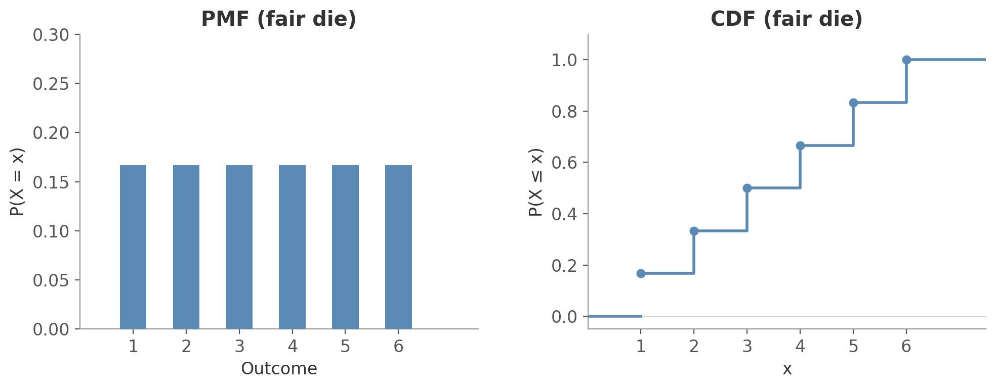 Figure 1: PMF and CDF for a fair die. Each bar is $1/6$; the CDF jumps by $1/6$ at each outcome.
For a continuous variable, the PDF shows the density curve and probabilities are areas under it. The CDF is the integral of the PDF - a smooth curve from 0 to 1:
 Figure 2: PDF and CDF for the standard normal. The shaded area on the left equals the probability $P(0.5 \leq X \leq 1.5)$. The CDF on the right shows $F(1.0) = 0.84$ - about 84% of values fall below 1.
| PMF (discrete) | PDF (continuous) | CDF (both) | |
|---|---|---|---|
| Answers | $P(X = x)$ | Density $f(x)$ | $P(X \leq x)$ |
| Question | “What’s the probability of exactly this value?” | “How dense is probability around this value?” | “What’s the probability of this value or less?” |
Key Distributions
Bernoulli Distribution (discrete)
The simplest distribution. One trial, two outcomes: success ($X = 1$) with probability $p$, failure ($X = 0$) with probability $1 - p$.
Notation: $X \sim \text{Bernoulli}(p)$
Or equivalently: $P(X = k) = p^k (1-p)^{1-k}, \quad k \in \{0, 1\}$
Properties:
$$\mathbb{E}[X] = P(X{=}1) \cdot 1 + P(X{=}0) \cdot 0 = p \cdot 1 + q \cdot 0 = p$$$$\text{Var}(X) = \mathbb{E}[X^2] - \mathbb{E}[X]^2 = p - p^2 = p(1-p)$$Your website has a 3% click-through rate on a banner ad. For any single visitor, this is a Bernoulli trial with $p = 0.03$: either they click ($X = 1$) or they don’t ($X = 0$).
The probability of no click: $P(X = 0) = (1 - 0.03)^1 = 0.97$.
Binomial Distribution (discrete)
Repeat a Bernoulli trial $n$ times independently. The binomial distribution counts the number of successes.
Notation: $X \sim \text{Binomial}(n, p)$
where $\binom{n}{k} = \frac{n!}{k!(n-k)!}$ is the binomial coefficient - the number of ways to choose which $k$ of the $n$ trials are successes.
Properties:
$$\mathbb{E}[X] = np$$$$\text{Var}(X) = np(1-p)$$Flip a fair coin 10 times. What’s the probability of exactly 7 heads?
$$P(X = 7) = \binom{10}{7} (0.5)^7 (0.5)^3 = 120 \times \frac{1}{1024} \approx 0.117$$About an 11.7% chance.
Poisson Distribution (discrete)
Counts the number of events in a fixed interval of time or space, when events occur independently at a constant average rate. Think: emails per hour, typos per page, server errors per day.
Notation: $X \sim \text{Poisson}(\lambda)$
where $\lambda$ is both the expected number of events and the rate parameter.
Properties:
$$\mathbb{E}[X] = \lambda$$$$\text{Var}(X) = \lambda$$Mean equals variance - a distinctive property of the Poisson. If you see data where the variance is much larger than the mean, the Poisson probably isn’t the right model.
A monitoring system logs an average of 4 errors per hour ($\lambda = 4$). What’s the probability of exactly 7 errors in the next hour?
$$P(X = 7) = \frac{4^7 e^{-4}}{7!} = \frac{16384 \times 0.0183}{5040} \approx 0.060$$About 6% - possible but uncommon. The expected count is 4, and 7 is nearly a standard deviation above that ($\sigma = \sqrt{\lambda} = 2$).
Uniform Distribution (continuous)
All values in an interval $[a, b]$ are equally likely. The simplest continuous distribution. (A discrete version exists too - the fair die from Figure 1 is a discrete uniform over $\{1, 2, 3, 4, 5, 6\}$.)
Notation: $X \sim \text{Uniform}(a, b)$
Properties:
$$\mathbb{E}[X] = \frac{a + b}{2}$$$$\text{Var}(X) = \frac{(b - a)^2}{12}$$A random number generator producing values between 0 and 1 follows $\text{Uniform}(0, 1)$. Wait times when you have no information about when the next bus arrives are often modelled as uniform.
A bus arrives every 15 minutes and you show up at a random time. Your wait time follows $\text{Uniform}(0, 15)$. The PDF is $f(x) = \frac{1}{15 - 0} = \frac{1}{15}$ for $0 \leq x \leq 15$. The probability you wait less than 5 minutes is the area under the PDF from 0 to 5:
$$P(X \leq 5) = \int_0^5 \frac{1}{15} \, dx = \frac{5 - 0}{15 - 0} = \frac{1}{3} \approx 0.333$$Your expected wait: $\mu = \frac{0 + 15}{2} = 7.5$ minutes. No matter when you arrive, on average you wait half the interval.
Exponential Distribution (continuous)
The flip side of the Poisson. Where Poisson counts how many events in a fixed interval, the exponential measures how long between consecutive events. If events happen at rate $\lambda$ per unit time, the count per interval is $\text{Poisson}(\lambda)$ and the wait between events is $\text{Exponential}(\lambda)$.
Notation: $X \sim \text{Exponential}(\lambda)$
Properties:
$$\mathbb{E}[X] = \frac{1}{\lambda}$$$$\text{Var}(X) = \frac{1}{\lambda^2}$$The exponential distribution is memoryless: $P(X > s + t \mid X > s) = P(X > t)$. The probability of waiting another $t$ minutes doesn’t depend on how long you’ve already waited.
If a server gets 4 requests per minute ($\lambda = 4$), the time between requests follows $\text{Exponential}(4)$. The expected wait is $1/\lambda = 0.25$ minutes (15 seconds). What’s the probability of waiting more than 30 seconds (0.5 minutes)?
$$P(X > 0.5) = e^{-4 \times 0.5} = e^{-2} \approx 0.135$$About 13.5%. The exponential is heavily right-skewed - most waits are short, but occasionally you get a long one.
Normal (Gaussian) Distribution (continuous)
The most important distribution in statistics. It shows up everywhere - not by coincidence, but because of the Central Limit Theorem (covered in the next post).
Notation: $X \sim \mathcal{N}(\mu, \sigma^2)$
Fully described by two parameters: $\mu$ (centre) and $\sigma$ (spread).
Properties:
$$\mathbb{E}[X] = \mu$$$$\text{Var}(X) = \sigma^2$$The formula looks intimidating, but the building blocks are intuitive:
- $e^{-x^2}$ gives you the bell shape - values far from 0 get exponentially less likely
- $(x - \mu)^2$ shifts the centre to $\mu$
- Dividing by $2\sigma^2$ controls the width - larger $\sigma$ means a wider, flatter bell
- $\frac{1}{\sigma\sqrt{2\pi}}$ is a normalizing constant so the area equals 1
Key properties:
- Symmetric around $\mu$
- About 68% of data falls within $\pm 1\sigma$, 95% within $\pm 2\sigma$, 99.7% within $\pm 3\sigma$ (the 68-95-99.7 rule)
- The sum of independent normals is also normal
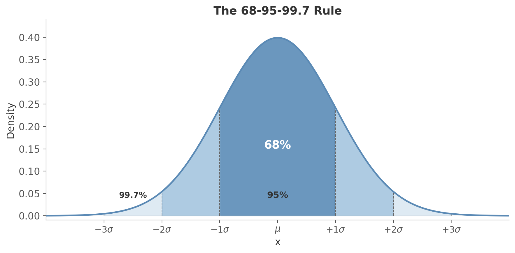 Figure 3: The 68-95-99.7 rule. The darkest region covers $\pm 1\sigma$ (68% of data), the medium region extends to $\pm 2\sigma$ (95%), and the lightest region reaches $\pm 3\sigma$ (99.7%).
Adult women’s heights in the US follow approximately $\mathcal{N}(161.3, 7.1^2)$ cm, meaning $\mu = 161.3$ and $\sigma = 7.1$. What fraction are taller than 175.5 cm?
How far is 175.5 from the mean, in units of $\sigma$?
$$175.5 - 161.3 = 14.2 = 2 \times 7.1 = 2\sigma$$So 175.5 cm is exactly $2\sigma$ above the mean. By the 68-95-99.7 rule, 95% of values fall within $\pm 2\sigma$, which means 5% fall outside that range. The normal distribution is symmetric, so half of that 5% is in each tail:
$$P(X > 175.5) = \frac{1 - 0.95}{2} = 0.025$$About 2.5% - roughly 1 in 40 women.
This worked out neatly because 175.5 landed exactly on $2\sigma$. For values that don’t, you’d look up the result in a z-table or compute it directly: scipy.stats.norm.sf(175.5, loc=161.3, scale=7.1).
Standard Normal and Z-Scores
The standard normal distribution has $\mu = 0$ and $\sigma = 1$. Any normal variable can be converted to it via standardization:
Converts any normal variable to the standard normal $\mathcal{N}(0, 1)$. The z-score tells you how many standard deviations $X$ is from the mean.
Say heights follow $\mathcal{N}(170, 7^2)$, so $\mu = 170$ and $\sigma = 7$. A person is 184 cm tall. How far from the mean is that, in standard deviations?
$$z = \frac{X - \mu}{\sigma} = \frac{184 - 170}{7} = \frac{14}{7} = 2$$A z-score of 2 means 184 cm is exactly 2 standard deviations above the mean. On the standard normal, this maps to the same position - $z = 2$.
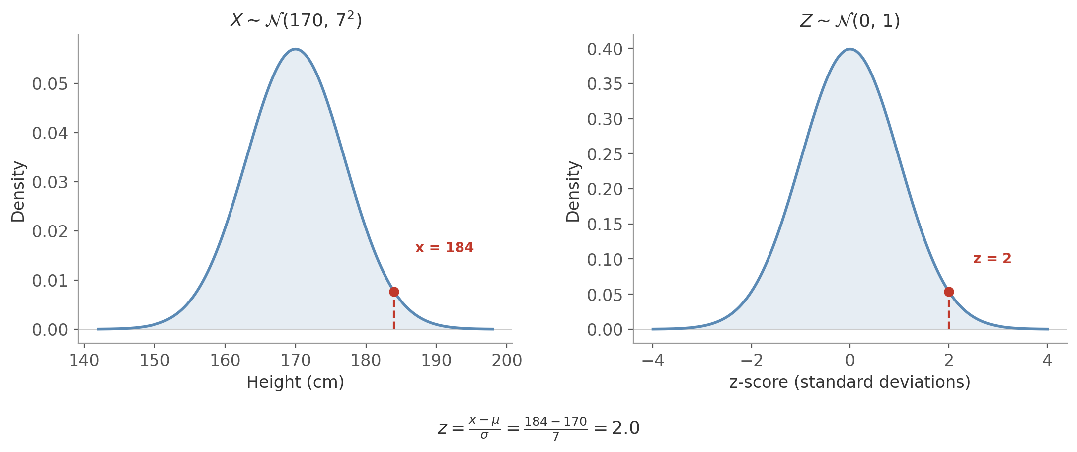 Figure 4: Standardization transforms $X \sim \mathcal{N}(170, 7^2)$ to $Z \sim \mathcal{N}(0, 1)$. The value $x = 184$ becomes $z = 2$ - the same relative position on both curves.
Standardization lets you compare variables measured on different scales - an exam score and a height measurement become comparable once expressed in standard deviations.
t-Distribution (continuous)
When you don’t know the population standard deviation $\sigma$ (which is almost always) and estimate it from the sample, the resulting statistic doesn’t follow a normal distribution - it follows a t-distribution.
Notation: $X \sim t(\nu)$
The t-distribution looks like a normal but with heavier tails - extreme values are more likely. It has one parameter: degrees of freedom ($\nu$), and as $\nu$ increases, the t-distribution converges to the standard normal.
Degrees of freedom ($\nu$): the number of independent pieces of information in your data that are free to vary.
Say you have 3 observations: 4, 7, 1. The mean is $\bar{x} = 4$. Now look at the deviations from the mean: $(4 - 4),\; (7 - 4),\; (1 - 4) = 0,\; 3,\; -3$. These always sum to zero - that’s a mathematical property of the mean, not a coincidence. So once you know any two of the deviations, the third is forced. Three observations, but only two free pieces of information.
In general: $n$ observations, one constraint (deviations sum to zero), so $\nu = n - 1$ degrees of freedom. You “spend” one degree of freedom estimating the mean, leaving $n - 1$ independent pieces of information to estimate the variance.
Why this matters for the shape: with few degrees of freedom, your estimate of $\sigma$ is unreliable. The t-distribution compensates by putting more probability in the tails - it’s saying “extreme values are more plausible because we’re not confident in our spread estimate.” As $\nu$ grows, the estimate of $\sigma$ stabilizes, the tails shrink, and the t-distribution becomes indistinguishable from the normal.
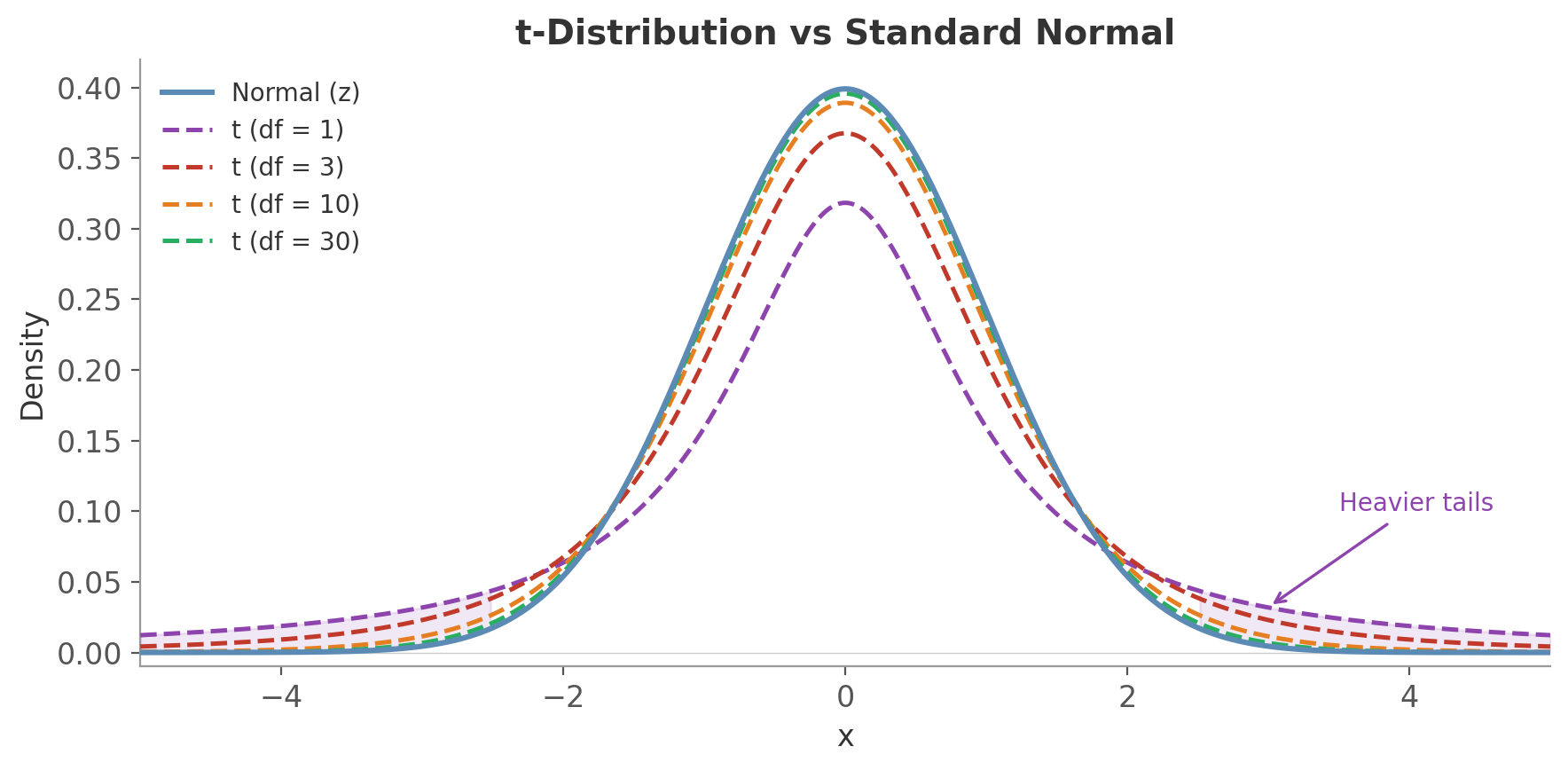 Figure 5: The t-distribution has heavier tails than the normal. With df = 1 the difference is dramatic; by df = 10 the curves are close; at df = 30 they’re nearly indistinguishable.
- Known $\sigma$, large $n$: use the normal distribution (z-scores)
- Unknown $\sigma$, any $n$: use the t-distribution (t-scores)
In practice, you almost always use the t-distribution. With $n > 30$ or so, the difference is negligible - but using $t$ is never wrong.
You measure the response time of 8 API calls and get $\bar{x} = 120\text{ms}$ with a sample standard deviation $s = 15\text{ms}$. Is the true mean plausibly 110ms?
With known $\sigma$, you’d compute a z-score: $z = \frac{120 - 110}{15 / \sqrt{8}} = 1.89$. Looking this up in the normal distribution, values beyond 1.89 have about 3% probability in each tail.
But you don’t know $\sigma$ - you estimated it from just 8 observations. So compute a t-score instead (same formula, different distribution):
$$t = \frac{\bar{x} - \mu_0}{s / \sqrt{n}} = \frac{120 - 110}{15 / \sqrt{8}} = 1.89$$Same number, but now look it up in the t-distribution with $\nu = 7$. The probability beyond 1.89 is about 5% per tail - noticeably higher than the normal’s 3%. The heavier tails reflect the fact that with only 8 observations, your estimate of the spread is uncertain.
With $n = 100$, the t-distribution with $\nu = 99$ gives essentially the same answer as the normal. The extra uncertainty only matters when $n$ is small.
We’ll use the t-distribution heavily in the next post. For now, the key idea: when $n$ is small and $\sigma$ is estimated, use $t$ instead of $z$ to account for the extra uncertainty.
Formula Reference
| Distribution | Type | PMF/PDF | Mean | Variance |
|---|---|---|---|---|
| $\text{Bernoulli}(p)$ | Discrete | $p^k(1-p)^{1-k}$ | $p$ | $p(1-p)$ |
| $\text{Binomial}(n, p)$ | Discrete | $\binom{n}{k}p^k(1-p)^{n-k}$ | $np$ | $np(1-p)$ |
| $\text{Poisson}(\lambda)$ | Discrete | $\frac{\lambda^k e^{-\lambda}}{k!}$ | $\lambda$ | $\lambda$ |
| $\text{Uniform}(a, b)$ | Continuous | $\frac{1}{b-a}$ | $\frac{a+b}{2}$ | $\frac{(b-a)^2}{12}$ |
| $\text{Exponential}(\lambda)$ | Continuous | $\lambda e^{-\lambda x}$ | $\frac{1}{\lambda}$ | $\frac{1}{\lambda^2}$ |
| $\text{Normal}(\mu, \sigma^2)$ | Continuous | $\frac{1}{\sigma\sqrt{2\pi}}e^{-\frac{(x-\mu)^2}{2\sigma^2}}$ | $\mu$ | $\sigma^2$ |
| $\text{t}(\nu)$ | Continuous | (complex) | $0$ | $\frac{\nu}{\nu - 2}$ |
Next up: the Law of Large Numbers and the Central Limit Theorem - what happens when you average enough samples, and why the normal distribution keeps showing up.