This is part 2 of the Math Foundations series.
Probability gives us a language for reasoning about uncertainty. Every time you train a model, run an A/B test, or compute a confidence interval, probability rules are doing the work underneath. This post covers the core building blocks.
Sample Space and Events
A sample space $\Omega$ is the set of all possible outcomes of an experiment. An event is a subset of the sample space - some collection of outcomes you care about.
Rolling a die: $\Omega = \{1, 2, 3, 4, 5, 6\}$. The event “roll an even number” is $\{2, 4, 6\}$.
Probability assigns a number between 0 and 1 to each event, measuring how likely it is.
The Three Axioms
All of probability theory rests on three axioms:
- Non-negativity: $P(A) \geq 0$ for any event $A$
- Normalization: $P(\Omega) = 1$ - something has to happen
- Additivity: if $A$ and $B$ are mutually exclusive (can’t both happen), then $P(A \cup B) = P(A) + P(B)$
Everything else - every formula in this post and the ones that follow - is derived from these three rules.
Complement Rule
The probability of an event not happening:
$$P(A') = 1 - P(A)$$If there’s a 30% chance of rain, there’s a 70% chance of no rain. Simple, but useful when it’s easier to compute the complement than the event itself.
Sum Rule
For two events that are mutually exclusive (disjoint - they can’t happen at the same time):
$$P(A \cup B) = P(A) + P(B)$$A coin flip is the simplest case: heads and tails are mutually exclusive. $P(\text{heads} \cup \text{tails}) = 0.5 + 0.5 = 1$.
For events that can overlap, we need to subtract the double-counted intersection:
$$P(A \cup B) = P(A) + P(B) - P(A \cap B)$$This is the inclusion-exclusion principle. Without the subtraction, outcomes in both $A$ and $B$ get counted twice.
Independence
Two events are independent if knowing one happened tells you nothing about the other. Formally:
$$P(A \cap B) = P(A) \times P(B)$$Flipping two coins: the first landing heads doesn’t affect the second. Drawing two cards with replacement - independent. Drawing two cards without replacement - not independent, because the first draw changes what’s left in the deck.
Independence is an assumption you make, not something you can always verify from data. In practice, many models assume independence for simplicity (Naive Bayes being the classic example) even when it’s not strictly true - and often still work well enough.
Conditional Probability
Conditional probability is the probability of $A$ given that $B$ has already happened:
$$P(A \mid B) = \frac{P(A \cap B)}{P(B)} \quad \text{(assuming } P(B) > 0\text{)}$$The intuition: once you know $B$ happened, $B$ becomes your new universe. You’re narrowing the sample space to only the outcomes where $B$ is true, then asking how many of those also include $A$.
A bag has 5 red and 3 blue marbles. You draw one and it’s red. What’s the probability the second draw (without replacement) is also red?
After the first draw, there are 4 red and 3 blue left - 7 total. So $P(\text{2nd red} \mid \text{1st red}) = \frac{4}{7}$.
Notice that conditional probability is where independence breaks down. If the events were independent, conditioning on $B$ wouldn’t change $P(A)$.
Bayes’ Theorem
Bayes’ theorem flips conditional probability around. If you know $P(B \mid A)$, you can compute $P(A \mid B)$:
This is directly derived from the conditional probability formula - no new assumptions.
The terms have names:
- $P(A)$: prior - your belief before seeing evidence
- $P(B \mid A)$: likelihood - how probable the evidence is if $A$ is true
- $P(A \mid B)$: posterior - your updated belief after seeing evidence
- $P(B)$: marginal likelihood - total probability of the evidence
Likelihood vs probability: these two words get used interchangeably in everyday language, but they mean different things here.
Probability $P(\text{data} \mid \theta)$: you’ve fixed the model parameters (i.e. the model is known), and you ask “what data/outcomes might I see?”
- Example: assuming a coin is fair ($\theta = 0.5$), what’s the probability of getting 7 heads in 10 flips?
Likelihood $L(\theta \mid \text{data})$: you’ve observed the data, and you ask “which model explains this best?”
- Example: I got 7 heads in 10 flips - is this coin fair ($\theta = 0.5$) or biased ($\theta = 0.7$)?
Mathematically they use the same formula, but the question is different. In probability, the parameters are known and the data is unknown. In likelihood, the data is known and the parameters are unknown.
This is exactly what maximum likelihood estimation (MLE) does in ML: given your training data, find the parameters $\theta$ that maximize $L(\theta \mid \text{data})$. When you train a logistic regression or fit a distribution, you’re searching for the $\theta$ that makes your observed data most probable.
In Bayes’ formula, $P(B \mid A)$ is called the likelihood because we’ve observed $B$ and we’re evaluating how probable that observation is under hypothesis $A$.
Law of Total Probability
To use Bayes’ theorem, you need $P(B)$ - the total probability of the evidence. If you don’t know it directly, you can compute it by summing over all possible hypotheses:
$$P(B) = P(B \mid A) \cdot P(A) + P(B \mid A') \cdot P(A')$$In plain terms: the total probability of seeing the evidence is the sum of “evidence when hypothesis is true” and “evidence when hypothesis is false,” each weighted by how likely that hypothesis is. This is how we compute the denominator in Bayes’ theorem.
Out of 1,000,000 people, 1 in 10,000 are sick - that’s 100 sick and 999,900 healthy. A test is 99% effective, i.e. it correctly identifies sick people 99% of the time and correctly identifies healthy people 99% of the time. You test positive.
What’s the probability you’re actually sick?
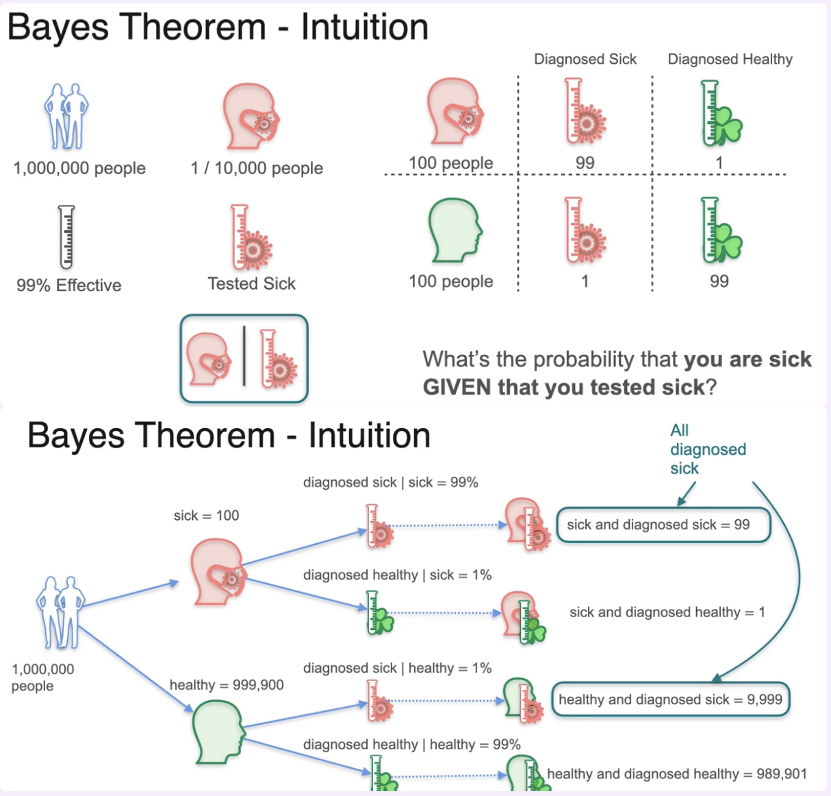 Figure 1: Bayes’ theorem - medical testing example
- $P(\text{sick}) = 0.0001$
- $P(\text{positive} \mid \text{sick}) = 0.99$
- $P(\text{positive} \mid \text{healthy}) = 0.01$
Work through the numbers:
- Of 100 sick people: 99 are correctly diagnosed sick, 1 is diagnosed healthy
- Of 999,900 healthy people: 9,999 are incorrectly diagnosed sick, 989,901 are correctly diagnosed healthy
Total diagnosed sick: $99 + 9{,}999 = 10{,}098$
Now apply Bayes - what’s the probability you’re actually sick, given you tested positive?
$$P(\text{sick} \mid \text{positive}) = \frac{99}{10{,}098} \approx 0.0098$$Less than 1%. A 99% accurate test, and you’re still almost certainly healthy. The prior is so low (1 in 10,000) that most positive results are false positives. This is why screening tests for rare conditions often require a second, more specific test.
Where Probability Meets ML
These rules show up everywhere in machine learning:
- Naive Bayes: applies Bayes’ theorem with the (naive) assumption that features are independent given the class. Often works surprisingly well despite the assumption being wrong.
- Logistic regression: models $P(Y = 1 \mid X)$ directly - given input features $X$, what’s the probability the outcome is positive? This is conditional probability: the prediction changes depending on what you condition on.
- A/B testing: uses probability to determine whether an observed difference is real or due to chance.
- Generative models: maximize the probability that generated outputs (images, text) resemble real data.
Formula Reference
| Rule | Formula |
|---|---|
| Complement | $P(A') = 1 - P(A)$ |
| Sum (disjoint) | $P(A \cup B) = P(A) + P(B)$ |
| Sum (general) | $P(A \cup B) = P(A) + P(B) - P(A \cap B)$ |
| Independence | $P(A \cap B) = P(A) \times P(B)$ |
| Conditional | $P(A \mid B) = \frac{P(A \cap B)}{P(B)}$ |
| Total probability | $P(B) = P(B \mid A) \cdot P(A) + P(B \mid A') \cdot P(A')$ |
| Bayes’ theorem | $P(A \mid B) = \frac{P(B \mid A) \cdot P(A)}{P(B)}$ |
Next up: Distributions & the Central Limit Theorem - the shapes data takes and why the normal distribution keeps showing up.