This is part 3 of the ML Fundamentals series.
Training a model is step one. Knowing whether it’s any good - and whether it will stay good on new data - is step two. The linear regression and regularization posts covered how to fit a model and control its complexity. This post covers the full evaluation toolkit: what to optimize during training (loss functions), what to report afterwards (metrics), and how to get honest estimates of performance (cross-validation and diagnostic curves).
Loss Functions
A loss function is the function the model minimizes during training. It defines what “good” means mathematically. Different tasks need different loss functions, and the choice shapes the model’s behavior.
Regression Losses
The average of squared differences between predicted and actual values.
Squaring does two things: it makes all errors positive, and it penalizes large errors disproportionately. An error of 10 contributes 100 to the sum, while an error of 1 contributes just 1. This means MSE is sensitive to outliers - a single wild prediction can dominate the loss.
MSE is the loss behind OLS regression and the default for gradient descent on regression problems. We saw it in the linear regression post as the cost function $J(\beta)$.
The average of absolute differences between predicted and actual values.
MAE treats all errors linearly. An error of 10 contributes exactly 10 times more than an error of 1. No disproportionate penalty, which makes it more robust to outliers.
The trade-off: MAE’s gradient is constant ($\pm 1$), which means it doesn’t naturally slow down near the minimum. Optimization can oscillate around the solution. MSE’s gradient shrinks as the error shrinks, making convergence smoother.
The choice depends on whether you care more about large errors or typical errors. Predicting house prices with some mansions in the dataset? MAE might be better - you don’t want a few luxury properties to dominate the loss. Predicting measurements where big errors are catastrophic? MSE, because it aggressively penalizes the worst predictions.
Huber Loss combines the best of both:
$$L_\delta = \begin{cases} \frac{1}{2}(y - \hat{y})^2 & \text{if } |y - \hat{y}| \le \delta \\ \delta|y - \hat{y}| - \frac{1}{2}\delta^2 & \text{if } |y - \hat{y}| > \delta \end{cases}$$Below the threshold $\delta$, it’s quadratic (smooth convergence like MSE). Above $\delta$, it’s linear (robust to outliers like MAE).
Classification Losses
where $y_i \in \{0, 1\}$ is the true label and $\hat{p}_i$ is the predicted probability of class 1.
Cross-entropy measures the distance between two probability distributions - the true labels and the model’s predicted probabilities. It penalizes confident wrong predictions heavily:
- True label is 1, model predicts $\hat{p} = 0.99$: loss is tiny ($-\log(0.99) \approx 0.01$)
- True label is 1, model predicts $\hat{p} = 0.01$: loss explodes ($-\log(0.01) \approx 4.6$)
The model gets severely punished for being confidently wrong.
This is the standard loss for logistic regression, neural networks, and any probabilistic classifier. It’s equivalent to negative log-likelihood, which means minimizing cross-entropy is the same as maximum likelihood estimation.
Hinge Loss takes a different approach:
$$L = \max(0,\; 1 - y_i \cdot f(x_i)) \quad \text{where } y \in \{-1, +1\}$$This is the loss behind SVMs. It only penalizes predictions that are on the wrong side of the margin or within it. Once a prediction is correct and confident enough (beyond the margin), the loss is zero - the model doesn’t care about making those predictions even more confident. This is why SVMs focus on the decision boundary rather than modeling probabilities.
Regression Metrics
Loss functions are for training. Metrics are for evaluation - they tell you and your stakeholders how the model performs in terms that make sense for the problem.
We defined R² in the linear regression post - here it is again as part of the evaluation toolkit.
The proportion of variance in $y$ explained by the model. The numerator is the model’s error; the denominator is the error you’d get by always predicting the mean.
$R^2 = 1.0$ means perfect predictions. $R^2 = 0$ means the model is no better than predicting the mean. It can go negative if the model is worse than the mean, which happens more often than you’d think with overfit models evaluated on new data.
$R^2$ never decreases when you add features, even useless ones. A random noise column will still nudge $R^2$ upward slightly on training data. Use adjusted $R^2$ for comparing models with different numbers of predictors.
where $n$ is the number of observations and $p$ is the number of predictors.
Adjusted $R^2$ penalizes model complexity. Unlike $R^2$, it can decrease when you add a feature that doesn’t improve the fit enough to justify its inclusion. If adding a variable bumps $R^2$ from 0.82 to 0.821 but adjusted $R^2$ drops, that variable isn’t earning its place.
RMSE (Root Mean Squared Error) is simply $\sqrt{MSE}$. It has the same units as $y$, which makes it interpretable as “typical error magnitude” - though it’s pulled upward by large errors, since it inherits MSE’s sensitivity to outliers.
MAE as a metric gives you a robust measure of the typical error. It’s the median-like counterpart to RMSE’s mean-like behavior.
MAPE (Mean Absolute Percentage Error) expresses errors as percentages of the actual values:
$$MAPE = \frac{1}{n}\sum_{i=1}^{n}\left|\frac{y_i - \hat{y}_i}{y_i}\right| \times 100\%$$This is popular in business and forecasting contexts because “the model is off by 8% on average” is easier to communicate than “RMSE is 4,200.” But MAPE has problems:
- Undefined when $y_i = 0$ - a single zero in the actuals breaks it
- Asymmetric - over-predictions can produce arbitrarily large percentage errors, but under-predictions are capped at 100%. Predicting 150 when actual is 100 gives 50%, but predicting 100 when actual is 150 gives only 33% - same absolute error, different MAPE
- Biased toward low predictions in optimization, since under-predicting produces smaller denominators
MdAPE (Median Absolute Percentage Error) replaces the mean with the median, making it robust to outliers. If a few predictions are wildly off, MdAPE won’t be dragged up the way MAPE is. Use it when your data has occasional extreme values but you still want percentage-based errors.
- RMSE: when large errors matter more than small ones
- MAE: for a robust “typical” error that isn’t inflated by outliers
- MAPE/MdAPE: when stakeholders need percentage-based errors (common in forecasting)
When in doubt, report both RMSE and MAE - they tell different stories, and the gap between them reveals how much outliers affect your model.
Classification Metrics
The Confusion Matrix
The confusion matrix is a 2x2 table that counts how the model’s predictions compare to reality. Every classification metric is derived from it.
| Predicted Positive | Predicted Negative | |
|---|---|---|
| Actually Positive | True Positive (TP) | False Negative (FN) |
| Actually Negative | False Positive (FP) | True Negative (TN) |
The rows are what actually happened. The columns are what the model said. The diagonal is where the model got it right.
The fraction of all predictions that are correct.
Accuracy is intuitive but deceptive.
A dataset where 95% of examples are negative gives 95% accuracy to a model that predicts “negative” every time. It has learned nothing. It catches zero positive cases. Accuracy hides this completely.
Precision, Recall, and F1
When classes are imbalanced - or when the costs of different errors are asymmetric - you need metrics that separate the two types of mistakes.
Precision: Of everything the model predicted positive, how many actually are?
$$\text{Precision} = \frac{TP}{TP + FP}$$High precision means few false alarms. When the model says “positive,” you can trust it. A spam filter needs high precision - sending a real email to spam (false positive) is worse than letting an occasional spam through.
Recall (also called Sensitivity or True Positive Rate): Of all actual positives, how many did the model find?
$$\text{Recall} = \frac{TP}{TP + FN}$$High recall means few missed positives. The model catches most of the real cases. A cancer screening tool needs high recall - missing a malignant case (false negative) is far worse than flagging a benign one for further testing.
Precision and recall are in tension. Push the classification threshold lower and you’ll catch more positives (higher recall), but you’ll also flag more negatives as positive (lower precision). Raise the threshold and precision improves, but recall drops.
It depends on the cost of each type of error:
- Optimize precision when false positives are costly: spam filtering, criminal sentencing, ad targeting (annoying users with irrelevant ads)
- Optimize recall when false negatives are costly: disease screening, fraud detection, security threats (missing a real threat is worse than a false alarm)
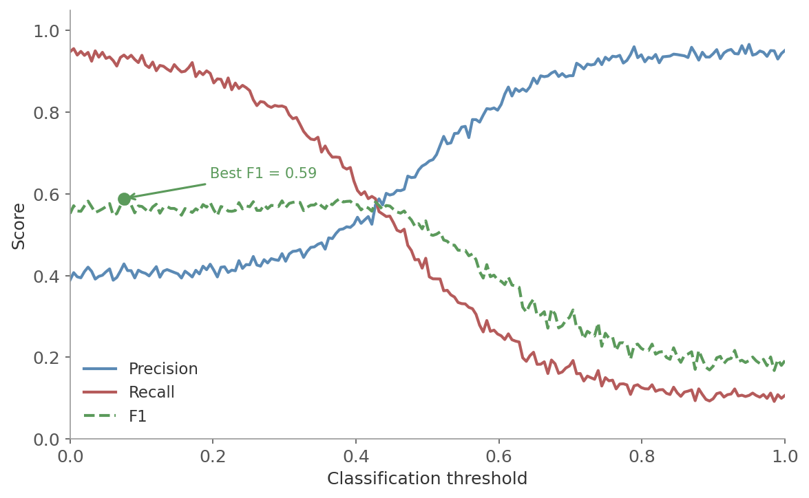 Figure 1: The precision-recall trade-off. As the classification threshold moves, precision and recall pull in opposite directions. The optimal threshold depends on which type of error is more costly.
The F1 Score combines precision and recall into a single number using the harmonic mean:
$$F1 = 2 \cdot \frac{\text{Precision} \cdot \text{Recall}}{\text{Precision} + \text{Recall}}$$The harmonic mean is appropriate here because it’s sensitive to low values. If either precision or recall is near zero, F1 is pulled down. A model with 95% precision and 10% recall gets F1 = 0.18, not the 52.5% that the arithmetic mean would give. F1 rewards balance between the two.
ROC Curve and AUC
Most classifiers output probabilities, not hard labels. The ROC curve (Receiver Operating Characteristic) shows how the model performs across all possible classification thresholds.
The axes:
- x-axis: False Positive Rate (FPR = FP/(FP + TN)) - the fraction of negatives incorrectly flagged
- y-axis: True Positive Rate (TPR = TP/(TP + FN)) - the fraction of positives correctly caught
Each point on the curve corresponds to a different threshold. Key landmarks:
- Top-left corner (TPR = 1, FPR = 0): perfect classifier
- Diagonal from (0,0) to (1,1): random classifier - catches positives and makes false alarms at the same rate
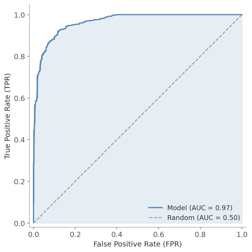 Figure 2: The ROC curve plots TPR against FPR at every possible threshold. The shaded area under the curve (AUC) summarizes overall performance. The dashed diagonal represents a random classifier (AUC = 0.5).
AUC (Area Under the ROC Curve) collapses the entire curve into a single number:
- AUC = 1.0: Perfect separation between classes
- AUC = 0.5: No discriminative ability (random guessing)
- AUC > 0.8: Generally considered good performance
The probabilistic interpretation: AUC is the probability that the model assigns a higher predicted score to a randomly chosen positive example than to a randomly chosen negative example. An AUC of 0.85 means that 85% of the time, a random positive gets a higher score than a random negative.
PR Curve and PR-AUC
The Precision-Recall curve plots precision against recall at every threshold - similar to the ROC curve, but focused on the positive class.
The axes:
- x-axis: Recall (TP/(TP + FN)) - how many positives did the model find?
- y-axis: Precision (TP/(TP + FP)) - of the predicted positives, how many are correct?
A perfect classifier sits in the top-right corner (precision = 1, recall = 1). A random classifier produces a horizontal line at $y = \text{prevalence}$ of the positive class.
PR-AUC (Area Under the PR Curve) summarizes the trade-off into a single number. Average Precision (AP) is a common approximation - it computes the weighted mean of precision at each threshold, with the weight being the increase in recall:
$$AP = \sum_k (R_k - R_{k-1}) \cdot P_k$$where $P_k$ and $R_k$ are precision and recall at the $k$-th threshold.
ROC-AUC can be misleading when you have very few positive examples. The FPR denominator (FP + TN) is dominated by true negatives, so even many false positives barely move the FPR - the ROC curve looks great while the model floods you with false alarms.
PR-AUC exposes this because precision drops directly when false positives increase. Use PR-AUC when the positive class is rare (fraud, disease, defects). Use ROC-AUC when classes are roughly balanced.
The Impact of Imbalanced Data
Class imbalance doesn’t just affect which metric you pick - it distorts the metrics themselves:
- Accuracy becomes meaningless. A 99% negative dataset gives 99% accuracy to a model that always predicts negative
- ROC-AUC stays artificially high because FPR barely moves when TN dominates
- Precision drops as false positives pile up among the many negatives
- Recall can look fine even for weak models if the threshold is low enough
What actually helps:
- Use PR-AUC, F1, or recall as your primary metric - they focus on the minority class
- Stratified splits for cross-validation (preserve class ratios in each fold)
- Class weights during training to penalize minority-class errors more heavily
- Resampling (oversampling the minority, undersampling the majority, or synthetic generation like SMOTE) - covered in a later post in this series
Multi-class Metrics
The metrics above assume binary classification. For multi-class problems, precision, recall, and F1 extend via averaging:
- Macro: compute the metric for each class independently, then average. Treats all classes equally regardless of size
- Micro: aggregate TP, FP, FN across all classes, then compute the metric. Dominated by the most common class
- Weighted: like macro, but weighted by each class’s support (number of examples). A good default for imbalanced multi-class problems
Scikit-learn’s classification_report shows per-class and averaged metrics side by side.
When to Use Which Metric
| Scenario | Recommended metric | Why |
|---|---|---|
| Balanced classes, simple evaluation | Accuracy | Straightforward, easy to communicate |
| Imbalanced classes | F1, PR-AUC | Accuracy hides poor minority-class performance |
| False positives are costly | Precision | Minimize false alarms |
| False negatives are costly | Recall | Minimize missed cases |
| Comparing models across thresholds | AUC-ROC | Threshold-independent comparison |
| Heavily imbalanced + threshold comparison | PR-AUC | AUC-ROC can be overly optimistic |
| Regression with outlier concern | MAE, MdAPE | Robust to extreme values |
| Regression where large errors matter | RMSE | Penalizes big misses |
| Regression with stakeholder reporting | MAPE | Percentage-based, easy to communicate |
| Regression model comparison | Adjusted $R^2$ | Accounts for model complexity |
Cross-Validation
You have a model and a metric. Now you need a reliable estimate of how the model will perform on new, unseen data. The simplest approach is a train-test split: train on 80%, test on 20%. But a single random split is noisy - a different split might give a noticeably different score. And you’re leaving 20% of your data unused for training.
Cross-validation solves both problems.
K-Fold Cross-Validation
Split the dataset into $k$ equally sized folds. Train the model on $k-1$ folds, evaluate on the remaining fold. Rotate which fold is held out and repeat $k$ times. Each observation appears in the test set exactly once.
The average of the $k$ individual fold scores. Report as mean $\pm$ standard deviation for a sense of variability.
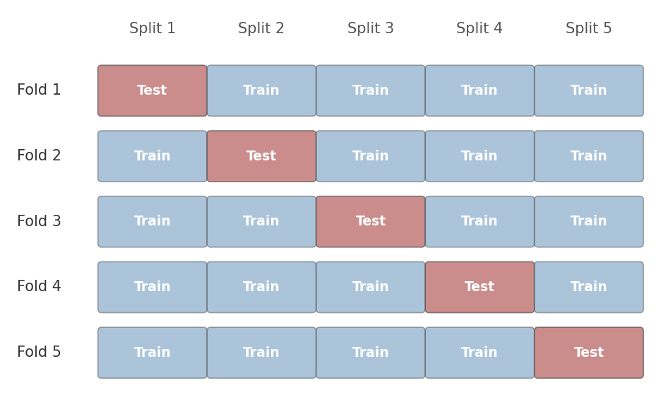 Figure 3: 5-fold cross-validation. In each iteration, one fold (shaded) serves as the test set and the remaining four are used for training. After five rounds, every observation has been tested exactly once.
$k = 5$ or $k = 10$ is standard. Larger $k$ means each training set is closer to the full dataset (less bias in the estimate) but the folds overlap more (higher variance between estimates, and higher computation cost).
Stratified K-Fold
Standard k-fold splits data randomly. If your dataset has 90% negative and 10% positive examples, a random fold might end up with 5% positives or 15% positives - neither is representative.
Stratified k-fold preserves the class proportions in each fold. If the full dataset is 90/10, every fold will be approximately 90/10. This is the default in scikit-learn’s cross_val_score for classification, and it should be the default in your head too. Always use stratified splits for classification with imbalanced classes.
Leave-One-Out (LOO)
The extreme case: $k = n$. Each fold contains a single observation. You train on $n-1$ examples and test on 1, repeated $n$ times.
LOO has low bias - each training set is nearly the full dataset. But it has high variance, because the $n$ training sets overlap almost entirely, making the individual estimates highly correlated. It’s also expensive: $n$ model fits instead of 5 or 10. Use it only for very small datasets where every data point matters.
Nested Cross-Validation
Here’s a subtle problem. Suppose you use 5-fold CV to compare several hyperparameter settings, pick the best one, and report that fold’s score as your expected performance. That score is biased upward - you selected it because it was the best among many options. It’s the same logic as looking at many p-values and reporting the smallest one.
Nested cross-validation fixes this with two loops:
- Inner loop: Runs k-fold CV to select the best hyperparameters (this is your model selection step)
- Outer loop: Runs k-fold CV to estimate the performance of the model selection process itself
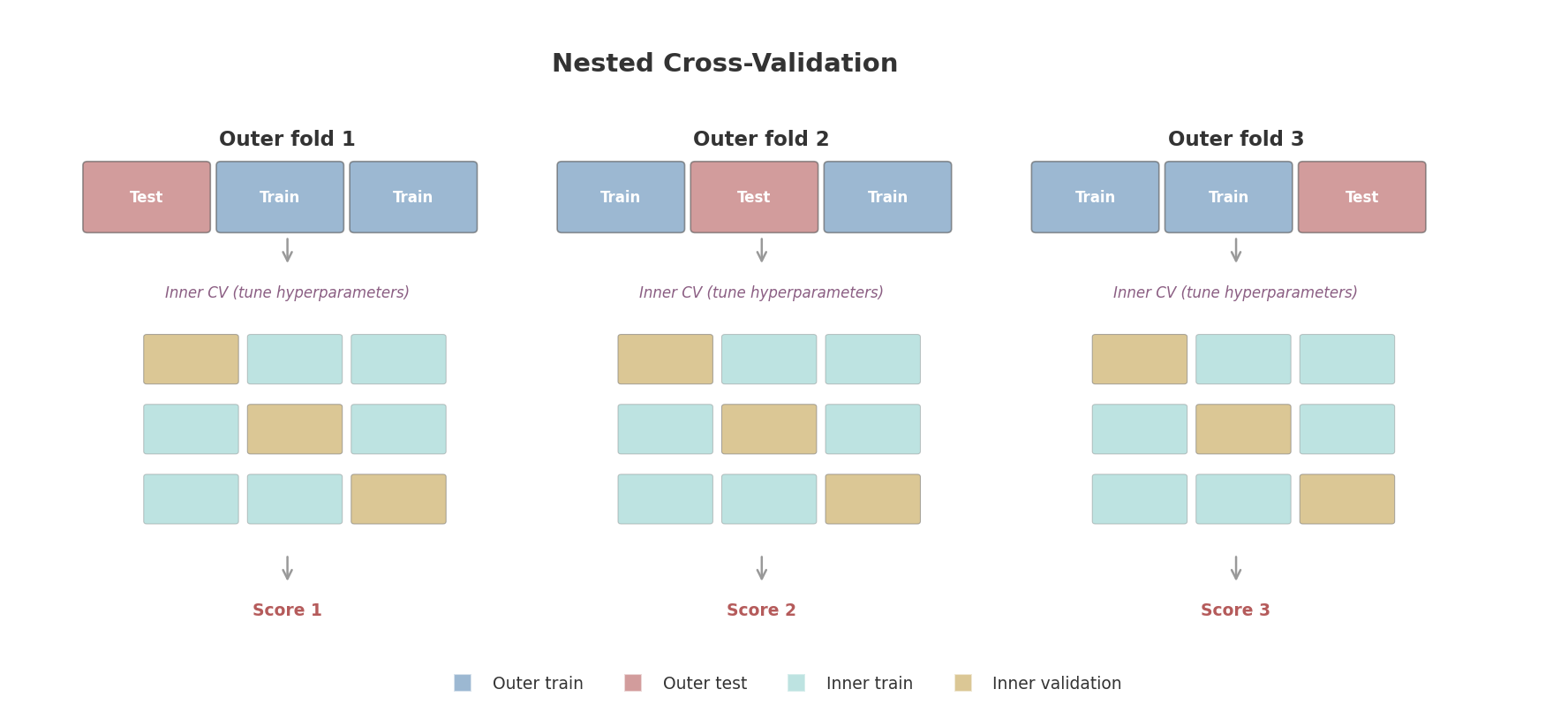 Figure 4: Nested cross-validation. The outer loop splits data into training and test folds. For each outer fold, the inner loop runs its own cross-validation on the training portion to tune hyperparameters. The outer test fold - never seen during tuning - gives an unbiased performance estimate.
If you tune hyperparameters on the same validation data you report results on, the estimate is biased upward. You’ve effectively “peeked” at the test data through the hyperparameter selection. Nested CV gives you an honest estimate of how well the entire pipeline - including hyperparameter tuning - will perform on truly unseen data.
The typical setup is 5-fold outer, 3-fold inner. The result is a performance estimate with uncertainty: “this modeling approach achieves F1 = 0.82 $\pm$ 0.03.” Once you have the estimate, retrain on all the data with the best hyperparameters for your final model.
Learning and Validation Curves
Cross-validation gives you a number. Learning and validation curves give you diagnostics - they help you understand why the model performs the way it does and what to do about it.
Learning Curves
A learning curve plots training and validation performance as a function of training set size. You train the model on 10% of the data, then 20%, then 30%, and so on, evaluating on a fixed validation set each time.
The two signatures to watch for:
High bias (underfitting):
- Both training and validation scores plateau at a low level, close together
- The model isn’t complex enough to capture the pattern
- More data won’t help - the model can’t learn anything more from what it already has
- Fix: a more complex model, additional features, or less regularization
High variance (overfitting):
- Training score is high but validation score is much lower, with a persistent gap
- The model memorizes the training data but doesn’t generalize
- More data will help - as the training set grows, the model learns the general pattern rather than specific noise
- Fix: regularization, simpler model, or more training data
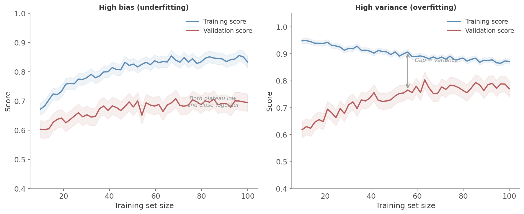 Figure 5: Learning curves for two scenarios. Left: high bias - both curves plateau low and close together. The model is too simple and more data won’t help. Right: high variance - the training score stays high while the validation score lags behind. More data or stronger regularization would close the gap.
Validation Curves
A validation curve plots training and validation performance as a function of a single hyperparameter. Instead of varying the amount of data, you vary the model’s complexity.
This reveals the sweet spot:
- Left side: both scores low - the model is too simple (underfitting)
- Right side: training score high but validation score drops - too complex (overfitting)
- Sweet spot: where the validation score peaks, before overfitting begins
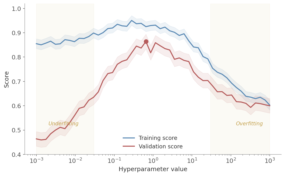 Figure 6: A validation curve for a regularization parameter. Left region: underfitting (both scores low). Middle: the sweet spot where validation performance peaks. Right region: overfitting (training score high, validation score falling).
These curves are cheap to produce in scikit-learn (learning_curve and validation_curve from sklearn.model_selection) and they save you from guessing. Before you reach for a bigger model or more data, check the curves. They’ll tell you whether that’s actually what you need.
Hyperparameter Tuning
Most models have hyperparameters - settings that aren’t learned from data but must be chosen beforehand. The regularization strength $\lambda$, the number of neighbors $k$, the tree depth. The right values depend on the specific dataset, so you search for them.
Grid Search
Grid search is the brute-force approach: specify a set of values for each hyperparameter and evaluate every combination with cross-validation.
- 3 values for $\lambda$ and 4 for $\alpha$: $3 \times 4 = 12$ combinations
- 5 hyperparameters with 10 values each: $10^5 = 100{,}000$ combinations
Simple and thorough, but the cost scales multiplicatively. Most combinations explore unimportant parts of the search space.
Randomized Search
Randomized search draws hyperparameter combinations randomly from specified distributions. Instead of an exhaustive grid, you set a budget - say 60 evaluations - and sample randomly.
With a budget of 60 trials, random search has a 95% chance of finding a combination in the top 5% of the search space. Grid search wastes trials on unimportant parameter combinations - if one hyperparameter matters much more than another, grid search still exhaustively explores the unimportant one. Random search naturally allocates more “coverage” along each dimension.
In practice, randomized search often finds equally good or better solutions than grid search, in a fraction of the time. It’s the better default choice, especially when you have more than two or three hyperparameters.
Halving Search
Successive halving is a more efficient strategy. Start with a large number of candidate configurations trained on a small subset of data. Evaluate them, discard the bottom half, and repeat with more data for the survivors. Each round halves the candidates and doubles the resources.
The logic: most bad configurations can be identified quickly with little data. Don’t waste a full cross-validation run on a clearly terrible hyperparameter setting. Save the expensive evaluations for the promising candidates.
Scikit-learn implements this as HalvingRandomSearchCV and HalvingGridSearchCV.
Practical Notes
Always maintain three separate data pools:
- Training data: for fitting the model
- Validation data (or cross-validation): for tuning hyperparameters and comparing models
- Test data: for the final, single evaluation at the end
The test set is touched once. If you go back and change the model after looking at test results, the test set is no longer unbiased.
Report metrics with uncertainty. A single number like “F1 = 0.85” hides how much that estimate varies. Report cross-validation results as mean $\pm$ standard deviation: “F1 = 0.85 $\pm$ 0.03 over 5 folds.” This tells the reader whether the model is consistently good or just good on average.
Choose metrics that match the problem. Default metrics are convenient but often wrong for your use case. A fraud detection system measured by accuracy will look great and catch nothing. Think about what kind of error matters more, then pick the metric that reflects that.
Use learning curves before adding complexity. If your model underfits, a bigger model might help but more data won’t. If it overfits, more data will help but a bigger model won’t. The curves tell you which situation you’re in. Five minutes of plotting can save hours of trying the wrong fix.
| Task | During training (loss) | After training (metric) | Validation method |
|---|---|---|---|
| Regression | MSE or Huber | RMSE, MAE, Adjusted $R^2$ | K-fold CV |
| Binary classification | Cross-entropy | F1, AUC-ROC, PR-AUC | Stratified k-fold CV |
| Imbalanced classification | Cross-entropy (with class weights) | F1, PR-AUC, Recall | Stratified k-fold CV |
| Model comparison | - | CV score $\pm$ std | Nested CV |
| Hyperparameter tuning | - | Validation curve, CV | Randomized or halving search |
Next in the ML Fundamentals series: decision trees and ensemble methods - from single trees to random forests and gradient boosting.