This is part 1 of the ML Fundamentals series.
The Math Foundations series built up the tools - distributions, sampling, the CLT, inference. Now we put them to use. Linear regression is where supervised learning starts: given input features, predict a continuous output. It’s simple enough to understand fully, practical enough to deploy, and foundational enough that most other models extend or rethink some piece of it.
The Model
Linear regression predicts a continuous outcome as a weighted sum of input features. In the simplest case - one feature, one output - the model is a straight line:
- $\beta_0$: the intercept - the predicted value when $x = 0$
- $\beta_1$: the slope - how much $y$ changes for a one-unit increase in $x$
- $\epsilon$: the error term - everything the model doesn’t capture
The goal is to find the values of $\beta_0$ and $\beta_1$ that make the predictions $\hat{y} = \beta_0 + \beta_1 x$ as close to the actual $y$ values as possible. “As close as possible” needs a precise definition - that’s what the cost function provides.
Fitting the Line: Ordinary Least Squares
Ordinary Least Squares (OLS) fits the line by minimizing the sum of squared residuals - the vertical distances between each data point and the line.
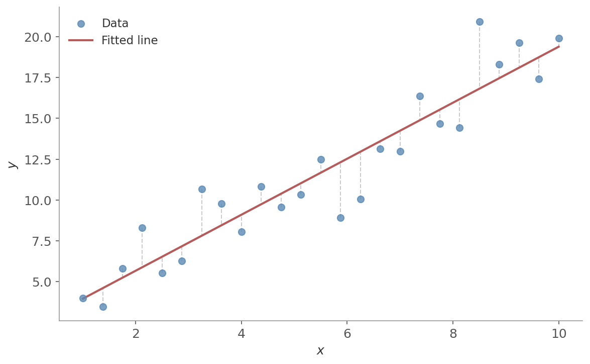 Figure 1: A fitted regression line through a scatter of data points. The vertical dashed lines show the residuals - the distances OLS minimizes. Points above the line have positive residuals, points below have negative ones.
The cost function is the Mean Squared Error (MSE):
$$J(\beta) = \frac{1}{n}\sum_{i=1}^{n}(y_i - \hat{y}_i)^2 = \frac{1}{n}\sum_{i=1}^{n}(y_i - \beta_0 - \beta_1 x_i)^2$$Setting the derivative of $J$ to zero and solving gives the normal equation - a closed-form solution:
where $X$ is the design matrix (features with a column of ones for the intercept) and $y$ is the vector of targets.
The geometric intuition:
- $\hat{y} = X\hat{\beta}$ is the projection of $y$ onto the column space of $X$
- OLS finds the point in that column space closest to $y$ in the Euclidean sense
- The residual vector $y - \hat{y}$ is perpendicular to the column space - that’s the orthogonality condition $X^T(y - X\hat{\beta}) = 0$, which is exactly the normal equation rearranged
import numpy as np
import matplotlib.pyplot as plt

x = np.array([1, 2, 3, 4, 5])
y = np.array([2.1, 3.8, 6.2, 7.9, 10.1])

# Design matrix: column of ones + feature
X = np.column_stack([np.ones_like(x), x])

# Normal equation
beta = np.linalg.inv(X.T @ X) @ X.T @ y
print(f"Intercept: {beta[0]:.2f}, Slope: {beta[1]:.2f}")
# Intercept: -0.01, Slope: 2.01

# Plot data and OLS fit
x_line = np.linspace(0.5, 5.5, 100)
plt.scatter(x, y)
plt.plot(x_line, beta[0] + beta[1] * x_line, color="red")
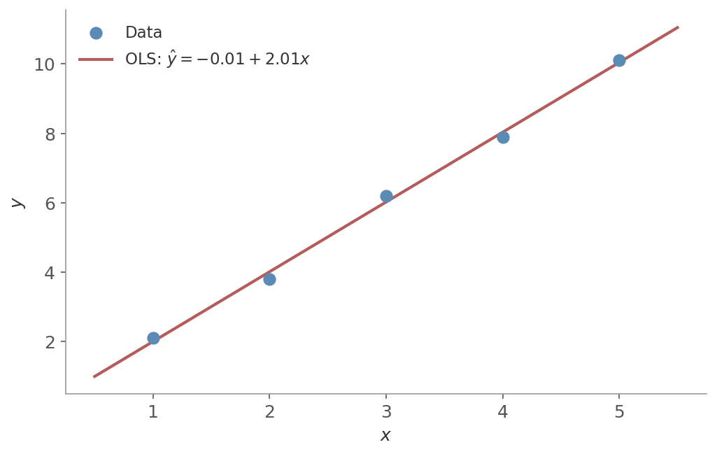 Figure 2: The normal equation recovers $\hat{y} \approx 2x$ from five data points. The closed-form solution finds the exact least-squares fit in one step - no iteration needed.
Gradient Descent
The normal equation requires computing $(X^TX)^{-1}X^T$, which scales as $O(p^3)$ where $p$ is the number of features. For large feature sets, that matrix inversion becomes expensive. Gradient descent avoids it entirely by iteratively updating the parameters in the direction that reduces the cost:
- Initialize the weights (zeros or small random values)
- Compute the gradient of the cost function: $\nabla J(\beta)$
- Update: $\beta \leftarrow \beta - \alpha \nabla J(\beta)$
- Repeat until convergence
The learning rate $\alpha$ controls the step size:
- Too large: updates overshoot the minimum, bouncing around or diverging
- Too small: convergence is painfully slow
- In practice: start with a reasonable value (0.01 is common) and adjust
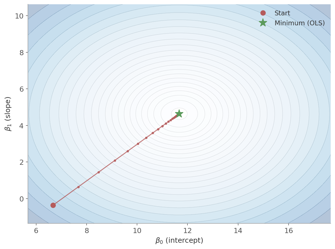 Figure 3: Gradient descent on the MSE surface. The contour lines show equal-cost regions. The red path starts far from the minimum and follows the steepest descent, eventually reaching the OLS solution (green star). Each dot is one update step.
Variants
| Variant | Uses per step | Pros | Cons |
|---|---|---|---|
| Batch | All $n$ examples | Stable, smooth convergence | Slow per step for large $n$ |
| SGD | 1 example | Fast updates, can escape local minima | Noisy, erratic path |
| Mini-batch | $b$ examples | Good balance of speed and stability | Extra hyperparameter |
In practice, mini-batch gradient descent is what most implementations use - it balances the stability of batch with the speed of SGD.
Data: $(x_1, y_1) = (1, 2)$ and $(x_2, y_2) = (2, 3)$. Model: $\hat{y} = \beta_0 + \beta_1 x$. Learning rate $\alpha = 0.1$. Start at $\beta_0 = 0, \beta_1 = 0$.
Batch computes one gradient using both points, then updates once:
- Predictions: $\hat{y}_1 = 0, \hat{y}_2 = 0$
- Gradients: $\frac{\partial J}{\partial \beta_0} = \frac{1}{2}[(0-2) + (0-3)] = -2.5$, $\;\frac{\partial J}{\partial \beta_1} = \frac{1}{2}[(0-2)(1) + (0-3)(2)] = -4$
- Update: $\beta_0 = 0 - 0.1(-2.5) = 0.25$, $\;\beta_1 = 0 - 0.1(-4) = 0.4$
SGD processes one point at a time, updating after each:
Point $(1, 2)$: $\hat{y} = 0$. Gradients: $-2, -2$. After update: $\beta_0 = 0.2, \beta_1 = 0.2$.
Point $(2, 3)$: now $\hat{y} = 0.2 + 0.2(2) = 0.6$. Gradients: $-2.4, -4.8$. After update: $\beta_0 = 0.44, \beta_1 = 0.68$.
After one pass: batch arrives at $(0.25, 0.4)$, SGD at $(0.44, 0.68)$. SGD moved further because it updated parameters between points - the second gradient was computed with already-updated weights. This is why SGD is noisier (each update uses partial information) but can converge faster (more updates per pass).
Feature scaling matters for gradient descent. If features are on very different scales, the cost surface is elongated and gradient descent zigzags instead of heading straight for the minimum. Standardizing features (zero mean, unit variance) makes the contours more circular and convergence faster.
Multiple Linear Regression
With more than one feature, the model becomes:
$$y = \beta_0 + \beta_1 x_1 + \beta_2 x_2 + \cdots + \beta_p x_p + \epsilon$$Or in matrix form: $y = X\beta + \epsilon$, where $X$ is an $n \times (p+1)$ design matrix - one row per observation, one column per feature plus a column of ones for the intercept.
Each coefficient $\beta_j$ represents the effect of feature $x_j$ on $y$, holding all other features constant. This is a key distinction from simple correlation. If you regress house price on both square footage and number of bedrooms, $\beta_1$ tells you the effect of adding one square foot while keeping bedrooms fixed.
The normal equation and gradient descent both work exactly the same way - only the dimensions change.
The Assumptions
Linear regression always produces coefficients. Whether those coefficients mean what you think they mean depends on a set of assumptions.
Linearity
The relationship between features and target is linear in the parameters. If the true relationship is quadratic and you fit a straight line, the residuals will show a systematic pattern.
How to check: Plot residuals vs fitted values. Random scatter around zero means linearity holds. A U-shaped curve means the model is missing curvature.
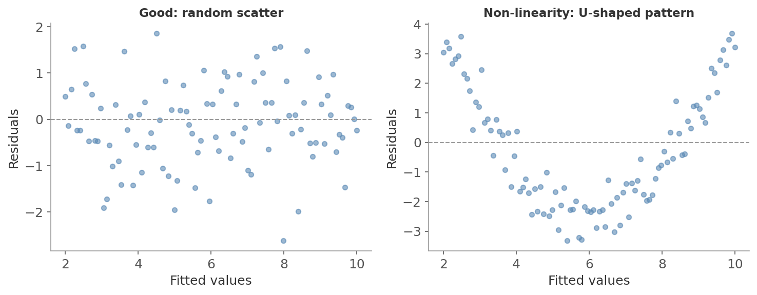 Figure 4: Left: good residuals - random scatter around zero, no pattern. Right: linearity violated - the U-shape shows the model misses curvature, with residuals systematically negative in the middle and positive at the edges.
Independence of Errors
The error from one observation should not be related to the error from another.
Imagine surveying 100 people about their income, but 50 of them are married couples who share finances. You don’t really have 100 independent observations - you have something closer to 75, because spouses’ incomes are related through shared economic circumstances. Correlated errors create the same problem in regression.
Why it matters:
- Standard errors become wrong. The formulas assume each data point contributes independent information. If errors are positively correlated, standard errors are artificially small - you’ll conclude effects are significant when they aren’t
- Your effective sample size is smaller than it appears. 1000 observations clustered into 100 groups with similar characteristics give you closer to 100 independent data points, not 1000
- Patterned residuals signal missing structure. If residuals follow a pattern (common in time series), the model is missing a variable or relationship
How to check: Plot residuals in observation order. Runs of the same sign indicate autocorrelation. The Durbin-Watson test formalizes this:
- Near 2: no autocorrelation
- Below 1.5: positive autocorrelation
- Above 2.5: negative autocorrelation
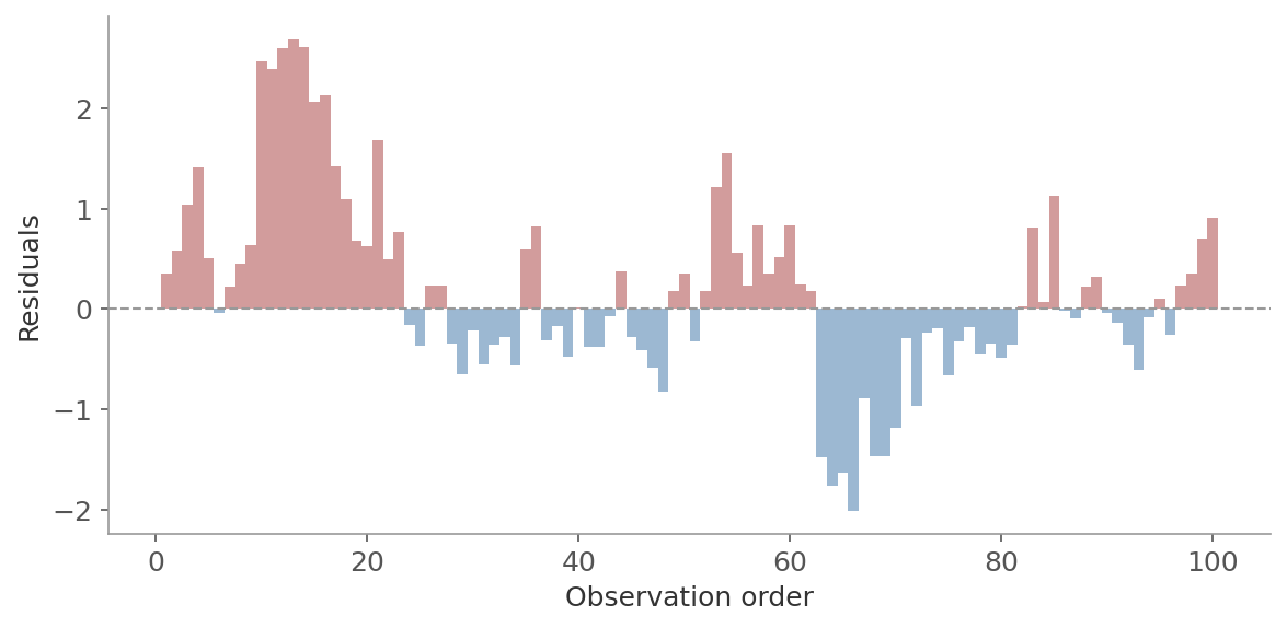 Figure 5: Residuals in observation order showing autocorrelation. Long runs of the same color (red = positive, blue = negative) mean successive errors are correlated rather than independent.
Homoscedasticity
The error variance should be constant across all values of $x$. If you see a funnel shape in a residuals vs fitted values plot - errors getting larger or smaller as predictions increase - this assumption is violated.
A classic example: income data. The variability in spending increases with income level. Low-income households have little discretionary spending variation, while high-income households show much more. Standard regression would incorrectly treat a 1,000 dollar prediction error the same whether it’s for someone earning 30,000 or 300,000 a year.
Why it matters:
- Standard errors become incorrect. The formulas assume constant error variance. If errors are larger for some predictions than others, standard errors will be wrong - sometimes too small, sometimes too large - making confidence intervals and p-values unreliable
- Hypothesis tests become invalid. Both t-tests and F-tests rely on constant variance. With heteroscedasticity, you can’t trust the significance of individual coefficients or the model as a whole
How to check: In a residuals vs fitted values plot, the vertical spread should be roughly constant. A widening funnel is the classic sign. The Breusch-Pagan test formalizes this by regressing squared residuals on the predictors.
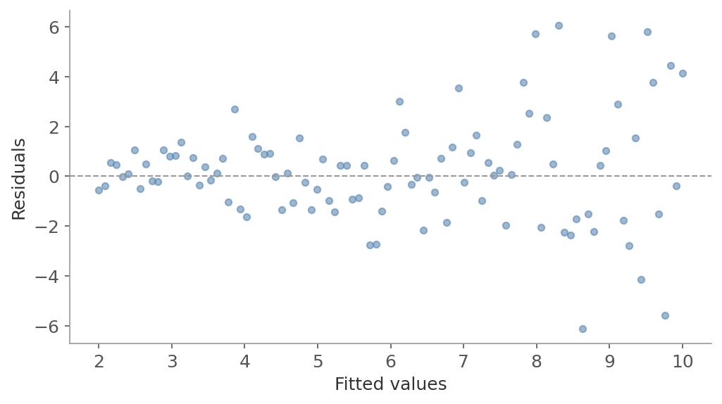 Figure 6: Heteroscedasticity - the funnel shape shows error variance increasing with fitted values. Points on the right scatter wider than on the left.
Normality of Errors
The residuals follow a normal distribution. This matters for inference - confidence intervals and p-values rely on it.
Normality of errors does not affect the coefficient estimates themselves. Under the first four assumptions (linearity, independence, homoscedasticity, no multicollinearity), OLS is BLUE - the Best Linear Unbiased Estimator (Gauss-Markov theorem). Normality only matters for statistical tests, not the fitted relationship.
For large samples, the CLT helps: even non-normal errors produce approximately normal coefficient distributions. If violated, options include:
- Variable transformations (log, square root)
- Robust regression
- Bootstrap methods
How to check: A Q-Q plot compares residual quantiles against theoretical normal quantiles. Points on the diagonal mean normality holds.
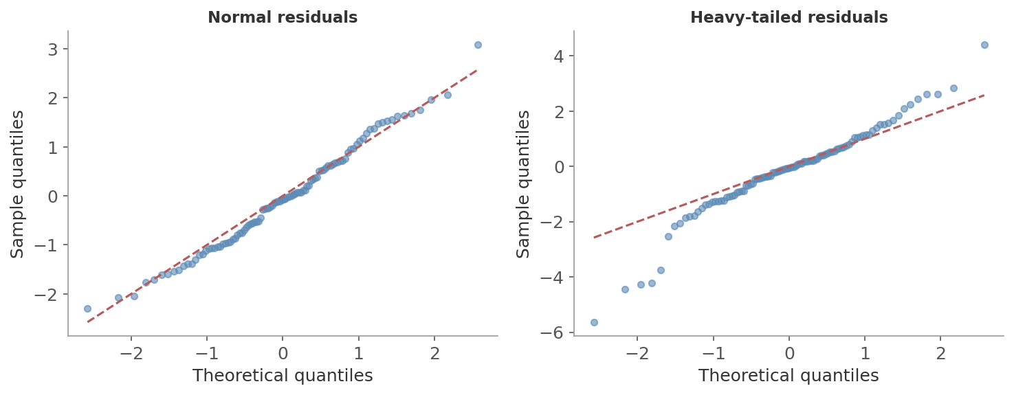 Figure 7: Left: normal residuals fall on the diagonal. Right: heavy-tailed residuals curve away at both ends - extreme values are more extreme than a normal distribution predicts.
No Multicollinearity
Independent variables should not be too highly correlated. When predictors are correlated, the model can’t tell which one deserves the credit, and coefficients become unstable.
Consider predicting house price with both square footage and number of rooms. These features are highly correlated - larger houses have more rooms. The model can’t separate their individual effects: it might assign a large positive coefficient to one and a small (or even negative) coefficient to the other, depending on small fluctuations in the data. The total prediction may still be reasonable, but the individual coefficients become meaningless.
Why it matters:
- Coefficients become unreliable. Small changes in the data can cause large swings in individual coefficient values, even flipping their signs
- Standard errors inflate. Correlated predictors make it harder to estimate each coefficient precisely, so confidence intervals widen and p-values increase - real effects can appear non-significant
How to check: The Variance Inflation Factor (VIF) measures how much a coefficient’s variance is inflated due to correlation with other predictors. A VIF above 5-10 is trouble. Remedies:
- Drop one of the correlated features
- Combine them (PCA)
- Use Ridge regularization
Evaluating the Fit
The proportion of variance in $y$ explained by the model. $RSS$ is the residual sum of squares; $TSS$ is the total sum of squares.
$R^2$ ranges from 0 to 1. A value of 0.75 means the model explains 75% of the variance in $y$. But $R^2$ never decreases when you add features - even useless ones - so it can be misleading for comparing models with different numbers of predictors.
Adjusted $R^2$ penalizes model complexity:
$$R^2_{adj} = 1 - \frac{(1-R^2)(n-1)}{n-p-1}$$Unlike $R^2$, adjusted $R^2$ can decrease when you add a feature that doesn’t improve the fit enough to justify its inclusion.
Residual Analysis
A good model leaves residuals that look like random noise:
- No pattern in a residual vs fitted values plot
- Roughly normal (check with a Q-Q plot)
- Constant spread across the range of fitted values
If you see structure in the residuals, the model is missing something - a non-linear relationship, a missing feature, or an interaction.
Statistical Tests
Regression estimates relationships - it gives you coefficients. But those coefficients come from a sample, so they carry sampling error. Statistical inference answers the follow-up question: are these estimates real, or could they be noise?
| What regression gives you | What inference tells you |
|---|---|
| Coefficient estimates | Whether the effect is real (p-values) |
| Predicted values | How uncertain predictions are (CIs) |
| Overall model fit | Whether the fit is significant (F-test, t-tests) |
The F-test asks whether the model as a whole explains more variance than you’d expect by chance. It compares explained variance per predictor to unexplained variance per residual degree of freedom:
where $p$ is the number of predictors and $n$ is the number of observations.
- $H_0$: all $\beta_j = 0$ (the model is no better than the mean)
- $H_1$: at least one $\beta_j \neq 0$
Interpreting the F-test:
- A high F-value and small p-value mean the model captures real signal
- A non-significant F-test means your predictors collectively don’t explain more than random noise - individual coefficient p-values shouldn’t be trusted in that case
- A model can have a decent $R^2$ and still fail the F-test if the sample is small or the number of predictors is large
$R^2$ tells you how much variance your model explains, but it describes only your sample. The F-test tells you whether that explanatory power is statistically meaningful or could have occurred by chance.
Individual Coefficients: t-tests
The t-test asks whether a single coefficient $\beta_j$ is significantly different from zero. The t-statistic is the coefficient divided by its standard error:
$$t_j = \frac{\hat{\beta}_j}{SE(\hat{\beta}_j)}$$- The p-value tells you whether the observed coefficient could have arisen by chance if the true coefficient were zero
- A non-significant coefficient doesn’t necessarily mean the feature is useless - it could be collinear with another feature, which inflates the standard error and makes the t-statistic small
Confidence and Prediction Intervals
Fitting gives you point predictions. Two types of interval quantify the uncertainty around them, and they answer different questions.
The confidence interval for the mean response at $x_0$ tells you where the regression line sits - how uncertain the estimated average $E[y \mid x_0]$ is:
$$\hat{y}_0 \pm t_{\alpha/2,\; n-p-1} \cdot \hat{\sigma}\sqrt{x_0^T(X^TX)^{-1}x_0}$$The prediction interval for a new observation at $x_0$ tells you where a single new data point is likely to fall:
$$\hat{y}_0 \pm t_{\alpha/2,\; n-p-1} \cdot \hat{\sigma}\sqrt{1 + x_0^T(X^TX)^{-1}x_0}$$The only difference is the $1 +$ under the square root - that’s the irreducible error variance. Even with perfect coefficient estimates, individual observations still scatter around the line, so the prediction interval is always wider.
Both intervals are narrowest near $\bar{x}$ and fan out toward the edges of the data - predictions far from the observed range carry more uncertainty.
Practical Notes
When to use linear regression:
- You need an interpretable model where coefficients have direct meaning
- As a baseline before trying anything more complex
- The relationship is approximately linear, or can be made so with feature transformations (log, polynomial terms)
When not to:
- The relationship is fundamentally non-linear and transformations don’t help
- Complex feature interactions matter and you can’t enumerate them manually
- Prediction accuracy matters more than interpretability
- Ignoring multicollinearity. Adding correlated features inflates standard errors and makes individual coefficients unreliable. Check VIF before interpreting coefficients.
- Using $R^2$ alone to evaluate. A model can have high $R^2$ on training data and still be useless on new data. Always check performance on held-out data, and look at residual plots rather than a single number.
With many features, OLS can overfit - the coefficients fit noise in the training data and predictions on new data suffer. Regularization (Ridge, Lasso, Elastic Net) addresses this by penalizing large coefficients. That’s the subject of the next post.
Next in the ML Fundamentals series: regularization and feature selection - preventing overfitting and choosing the right features.