Hypothesis Testing, Confidence Intervals and Power

This is part 5 of the Math Foundations series.

The CLT gave us the sampling distribution - the sample mean is approximately normal, centred at $\mu$, with spread $SE = s / \sqrt{n}$. This post turns that into a decision-making framework: how to state a claim, test it against data, quantify uncertainty, and plan how much data you need.

Hypothesis Testing

Null and Alternative Hypotheses

Every hypothesis test starts with two competing statements about a population parameter.

Hypotheses

Null hypothesis ($H_0$): the default claim. Usually “no effect” or “no difference.”

Alternative hypothesis ($H_1$): what you’re trying to find evidence for.

$$H_0: \mu = \mu_0 \quad \text{vs.} \quad H_1: \mu \neq \mu_0$$

The logic is indirect. You don’t prove $H_1$ - you ask whether the data are unlikely enough under $H_0$ to reject it.

One-Sided vs Two-Sided Tests

The alternative hypothesis determines where you look for evidence against $H_0$:

Two-sided (two-tailed): $H_1: \mu \neq \mu_0$. Reject if the test statistic falls in either tail. The rejection region is split: $\alpha/2$ in each tail.
One-sided (one-tailed): $H_1: \mu > \mu_0$ or $H_1: \mu < \mu_0$. All of $\alpha$ goes into one tail - easier to reject in that direction, but you can’t detect effects in the other.

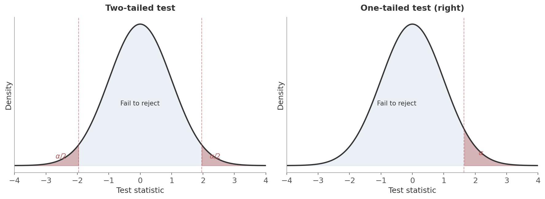$One-sided vs two-sided rejection regions$ Figure 1: Two-tailed (left) vs one-tailed (right) rejection regions. The red shaded areas are the rejection regions - if the test statistic lands there, you reject $H_0$. A two-tailed test splits $\alpha$ across both tails; a one-tailed test puts all of $\alpha$ in one tail.

Use two-sided unless you have a strong reason to only care about one direction before seeing the data. In A/B testing, for instance, you often use one-sided because you only care whether the variation is better than the control. But if a change could make things worse and you want to detect that too, use two-sided.

Test Statistics

A test statistic converts your data into a single number that you can compare against a known distribution. The idea: if $H_0$ is true, this number should look like a typical draw from that distribution. If it’s unusually far out, $H_0$ is in trouble.

One-sample t-statistic

$$t = \frac{\bar{x} - \mu_0}{s / \sqrt{n}}$$

Numerator: how far the sample mean is from the hypothesised value
Denominator: the standard error - expected sampling variability
Ratio: how many standard errors away from $\mu_0$ your data landed

Two-sample t-statistic (Welch's t-test)

$$t = \frac{\bar{x}_1 - \bar{x}_2}{\sqrt{\frac{s_1^2}{n_1} + \frac{s_2^2}{n_2}}}$$

with degrees of freedom:

$$df = \frac{\left(\frac{s_1^2}{n_1} + \frac{s_2^2}{n_2}\right)^2}{\frac{(s_1^2/n_1)^2}{n_1 - 1} + \frac{(s_2^2/n_2)^2}{n_2 - 1}}$$

Same logic: difference in means divided by the standard error of that difference. The $df$ formula (Welch-Satterthwaite) looks messy but it just accounts for potentially unequal variances and sample sizes.

Proportion z-statistic

$$z = \frac{\hat{p} - p_0}{\sqrt{\frac{p_0(1 - p_0)}{n}}}$$

For comparing two proportions (e.g. conversion rates in an A/B test), pool them under $H_0$:

$$z = \frac{\hat{p}_1 - \hat{p}_2}{\sqrt{\hat{p}(1 - \hat{p})\left(\frac{1}{n_1} + \frac{1}{n_2}\right)}} \quad \text{where } \hat{p} = \frac{x_1 + x_2}{n_1 + n_2}$$

$x_1, x_2$: number of successes (e.g. conversions) in each group
$\hat{p}$: pooled proportion - overall success rate across both groups, used because under $H_0$ we assume the two proportions are equal

Same structure as the t-statistic: observed difference divided by standard error.

z-test vs t-test: when to use which

For means, use the t-test. It handles unknown population variance (which is almost always the case), and with large $n$ the t-distribution converges to the normal anyway. You lose nothing by defaulting to t.

For proportions, use the z-test. The variance under $H_0$ is fully determined by $p_0$ (since $\text{Var} = p_0(1-p_0)/n$), so there’s no unknown variance to estimate. The z-test is the standard choice.

P-Values

P-value

The p-value is the probability of observing a test statistic as extreme as (or more extreme than) the one you got, assuming $H_0$ is true.

Two-sided: $p = P(|T| \geq |t_{obs}| \mid H_0)$ - extreme in either direction
One-sided: $p = P(T \geq t_{obs} \mid H_0)$ - extreme in one direction only

The logic, step by step:

Assume there’s no real effect ($H_0$ is true)
Under that assumption, the CLT tells you what the sampling distribution looks like
Compute where your data falls on that distribution
The p-value is the probability of landing that far out or farther

A small p-value means your data would be unusual if $H_0$ were true - which is evidence against $H_0$.

Example: is this coin fair?

A friend hands you a coin and claims it’s fair. You’re not so sure, so you flip it 10 times and get 9 heads. Should you believe your friend?

Take their claim as the null hypothesis:

$H_0$: the coin is fair ($p = 0.5$)
$H_1$: the coin is not fair ($p \neq 0.5$)

If your friend is right, the number of heads $X$ follows $\text{Binomial}(10, 0.5)$. The p-value asks: how likely is a result this extreme or more, if the coin really is fair? You got 9 heads, so $P(X \geq 9) = P(X = 9) + P(X = 10)$. But since you’d be equally suspicious of 9 tails, this is a two-sided test - you also count the mirror extreme, $P(X \leq 1) = P(X = 0) + P(X = 1)$. By symmetry of the fair coin, both tails are equal:

$$p = P(X \leq 1) + P(X \geq 9) = 2 \times \frac{\binom{10}{9} + \binom{10}{10}}{2^{10}} = 2 \times \frac{10 + 1}{1024} \approx 0.021$$

Only about 2% of the time would a fair coin produce something this lopsided. At $\alpha = 0.05$, you’d reject your friend’s claim. You haven’t proven the coin is biased - but the data is hard to explain if it’s fair.

The p-value is not

The probability that $H_0$ is true. It’s $P(\text{data} \mid H_0)$, not $P(H_0 \mid \text{data})$.
The probability the result happened “by chance.” It’s the probability of data this extreme under a specific null model.
A measure of effect size. A tiny difference can produce a small p-value with enough data. A large difference can produce a large p-value with too little.

Significance Level and Decisions

Significance level

The significance level $\alpha$ is the threshold you set before looking at the data.

If $p \leq \alpha$: reject $H_0$
If $p > \alpha$: fail to reject

The standard choice is $\alpha = 0.05$ - a 5% chance of a false positive. The connection to confidence intervals: $\alpha = 1 - \text{confidence level}$, so 95% CI $\leftrightarrow$ $\alpha = 0.05$.

Type I and Type II Errors

A hypothesis test can be wrong in two ways:

Type I error (false positive):

You reject $H_0$ when it’s actually true
The coin is fair, you just got an unlucky streak
Probability: $\alpha$

Type II error (false negative):

You fail to reject $H_0$ when it’s actually false
The coin is biased, but your 10 flips weren’t extreme enough to catch it
Probability: $\beta$

Think of a fire alarm. Positive/negative refers to the alarm (did it go off or not), false means it was wrong:

False positive: alarm goes off, no fire. You “detected” something that isn’t there.
False negative: no alarm, building is on fire. You missed something real.

"Fail to reject" is not "accept"

Failing to reject $H_0$ means the data didn’t provide strong enough evidence against it. It doesn’t mean $H_0$ is true. You might simply not have enough data. Think of it like a jury verdict: “not guilty” doesn’t mean “innocent” - it means the evidence didn’t meet the standard.

Worked Example - One-Sample t-Test

Example: website session duration

A website’s historical average session duration is $\mu_0 = 30$ minutes. After a redesign, you sample $n = 50$ sessions and observe $\bar{x} = 33.2$ minutes with $s = 12.5$ minutes. Did the redesign change session duration?

Step 1: State hypotheses.

$$H_0: \mu = 30 \quad \text{vs.} \quad H_1: \mu \neq 30$$

(Two-sided - the redesign could increase or decrease duration.)

Step 2: Compute the test statistic.

$$t = \frac{33.2 - 30}{12.5 / \sqrt{50}} = \frac{3.2}{1.768} = 1.81$$

Step 3: Find the p-value. With $df = 49$ and a two-tailed test:

$$p = 2 \times P(t_{49} > 1.81) = 2 \times 0.038 = 0.076$$

Step 4: Decide. At $\alpha = 0.05$: $p = 0.076 > 0.05$, so we fail to reject $H_0$. The data don’t provide sufficient evidence that the redesign changed session duration.

Note: at $\alpha = 0.10$, we would reject. The threshold matters.

Confidence Intervals

The CLT post covered the mechanics - the formula, the visualization, what “95% confidence” means across repeated samples. This section adds what that post didn’t: interpretation pitfalls, what controls width, and the connection to hypothesis testing.

Interpretation

Correct interpretation

“If we repeated this sampling procedure many times, about 95% of the resulting intervals would contain the true parameter.”

Common misconception

“There’s a 95% probability that the true value is in this interval.”

The difference is subtle but real. Once you’ve computed the interval, the true parameter is either in it or it isn’t - there’s no probability involved. The “95%” refers to the long-run success rate of the procedure, not to any single interval.

What Controls CI Width

Three levers determine how wide a confidence interval is:

Margin of error

$$\text{Margin of error} = t^* \cdot \underbrace{\frac{s}{\sqrt{n}}}_{\text{SE}}$$

where $t^*$ is the critical value for the chosen confidence level (e.g. $t^* \approx 1.96$ for 95% with large $n$).

Sample size ($n$): more data $\to$ smaller SE $\to$ narrower CI. The $\sqrt{n}$ means diminishing returns - quadruple the data to halve the margin.
Variability ($s$): noisier data $\to$ wider CI. You can’t control this, but you can sometimes reduce it with better measurement or stratification.
Confidence level: higher confidence $\to$ wider CI. A 99% interval is wider than a 95% interval from the same data. You’re casting a wider net to be more sure you catch the true value.

CIs and Hypothesis Tests Are the Same Thing

A confidence interval and a hypothesis test answer the same question from different angles:

Hypothesis test: can I reject this specific value?
Confidence interval: here are all the values you can’t reject

The 95% CI is $\bar{x} \pm 1.96 \times SE$:

$\mu_0$ inside the interval $\to$ $p > 0.05$ $\to$ can’t reject
$\mu_0$ outside the interval $\to$ $p \leq 0.05$ $\to$ reject

Say you’re testing whether a new feature changes average session time ($H_0: \mu_1 - \mu_2 = 0$). You compute the 95% CI for the difference:

CI is $[-0.8, 1.4]$: contains 0. No effect is a plausible value - can’t reject $H_0$.
CI is $[0.3, 2.1]$: excludes 0. Every plausible value is positive - reject $H_0$. The effect is somewhere between 0.3 and 2.1.

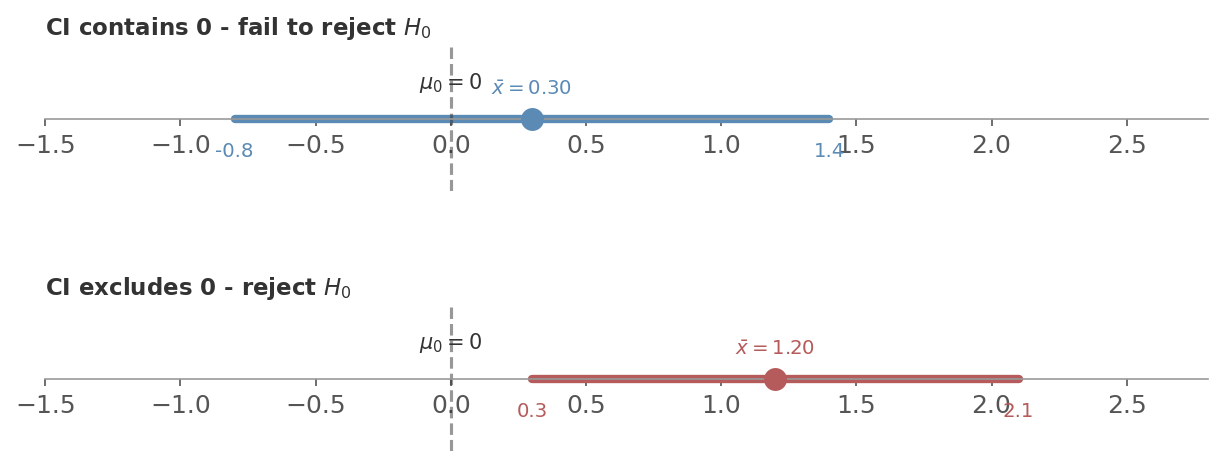$CI and hypothesis test duality$ Figure 2: The CI-hypothesis test duality. Top: the 95% CI $[-0.8, 1.4]$ contains 0, so we fail to reject $H_0$. Bottom: the CI $[0.3, 2.1]$ excludes 0, so we reject $H_0$. Same information, two views.

This is why many statisticians prefer reporting CIs over p-values. A p-value tells you “significant or not.” A CI tells you that and gives the plausible range of the true effect - something the p-value alone doesn’t give you.

CIs and Power

The width of a confidence interval tells you how much power you have. The chain works like this:

The 95% CI is $\bar{x} \pm 1.96 \times SE$, and $SE = s / \sqrt{n}$
Wide CI = large uncertainty. If the true effect is small, the interval will probably still contain 0 - you’ll miss it. That’s low power.
Narrow CI = high precision. Even a small true effect pushes the interval away from 0. That’s high power.
More data shrinks $SE$, which narrows the CI, which increases power.

Back to the session-time example. Say the true effect of your new feature is a 1-minute increase ($\sigma = 3$). Watch what happens as you increase the sample size:

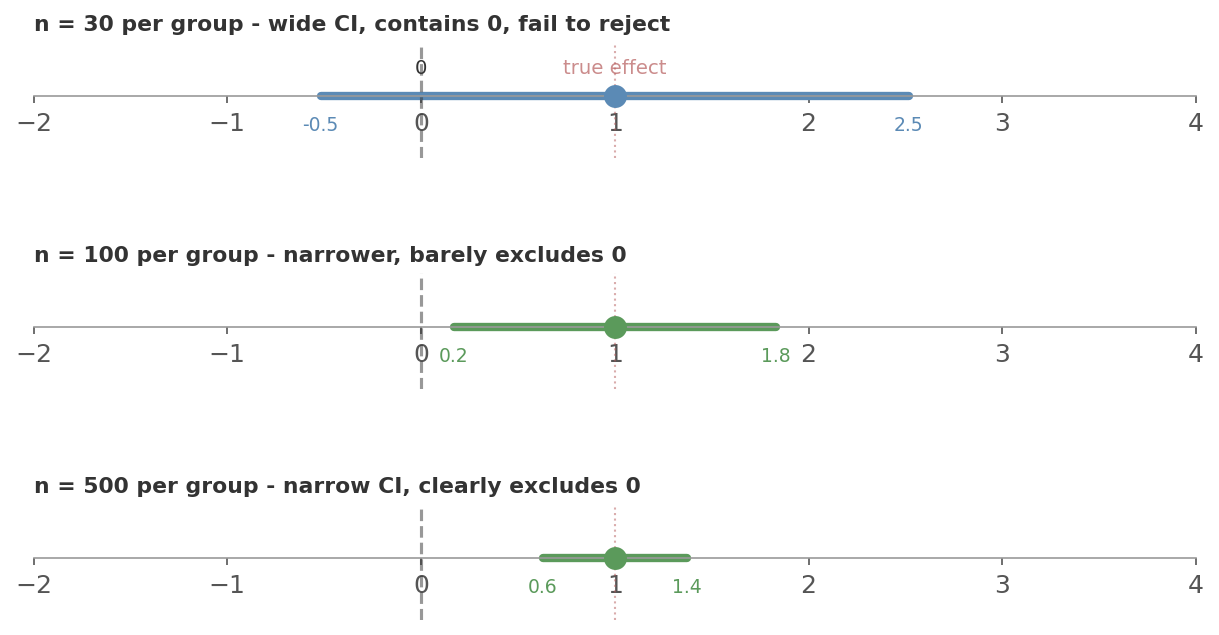$CI width and power$ Figure 3: The same true effect (dotted red line), three different sample sizes. With $n = 30$ per group the CI (blue) is wide enough to contain 0 - you fail to reject and miss the real effect. At $n = 100$ the CI (green) barely excludes 0. At $n = 500$ it’s narrow and clearly excludes 0. The effect didn’t change. Your precision did.

In short: wider CI means lower power, narrower CI means higher power. Collecting more data does both at once - it shrinks the CI and increases the probability of detecting a real effect.

Power Analysis and Sample Size

Statistical Power

Power is the probability of correctly rejecting $H_0$ when it’s actually false - detecting a real effect when one exists.

$$\text{Power} = 1 - \beta = P(\text{reject } H_0 \mid H_1 \text{ is true})$$

The convention is to aim for power $\geq 0.80$, meaning at least an 80% chance of detecting the effect if it’s real. That still leaves a 20% chance of missing it.

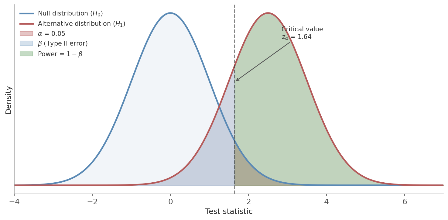$Statistical power diagram$ Figure 4: The canonical power diagram. The blue curve is the sampling distribution under $H_0$ (no effect). The red curve is the distribution under $H_1$ (real effect of size $d$). The dashed line is the critical value. The red shaded area in the right tail of the null is $\alpha$ (Type I error). The blue shaded area to the left of the critical value under the alternative is $\beta$ (Type II error - failing to detect a real effect). The green area is power: the probability of correctly rejecting $H_0$ when the effect is real.

Two ways to increase power (green area):

Larger effect - moves the alternative distribution further right
Larger $\alpha$ - moves the critical value left, but at the cost of more false positives

Effect Size

The raw difference between means depends on the scale of measurement - a 2-point difference means something different for SAT scores than for a 5-point survey. Effect size standardises this by dividing by the standard deviation.

Cohen's d

$$d = \frac{\bar{x}_1 - \bar{x}_2}{s_p}$$

where $s_p$ is the pooled standard deviation. Cohen’s conventions:

$d$	Interpretation
0.2	Small
0.5	Medium
0.8	Large

These are rough guidelines, not rules. A “small” effect in one context can be practically important in another.

Minimum Detectable Effect (MDE)

In A/B testing, you don’t usually think in terms of Cohen’s $d$. Instead, you specify the minimum detectable effect - the smallest difference that would be practically meaningful. “We want to detect at least a 2 percentage point increase in conversion rate.” The MDE is the same idea as effect size, just in the original units rather than standardised.

The Four-Way Trade-off

Four quantities are linked: $\alpha$, power, effect size, and sample size. Fix any three and the fourth is determined.

Want to detect smaller effects? You need more data.
Want higher power? You need more data (or accept a larger $\alpha$).
Want a stricter $\alpha$? You need more data (or accept lower power).

The sample size formula for a two-sample test (equal groups) makes this explicit:

Sample size per group

$$n = \frac{(z_{\alpha/2} + z_{\beta})^2 \cdot 2s^2}{\delta^2}$$

$\delta$: minimum detectable difference
$s$: assumed standard deviation
$z_{\alpha/2}$: critical value for the significance level
$z_{\beta}$: critical value for the desired power

Example: sample size calculation

You’re planning an A/B test on session duration. Current average is 30 minutes with $s = 18$ minutes. You want to detect a 3-minute increase ($\delta = 3$) with 80% power at $\alpha = 0.05$.

$z_{\alpha/2} = z_{0.025} = 1.96$ (two-tailed)
$z_{\beta} = z_{0.20} = 0.84$ (80% power)

$$n = \frac{(1.96 + 0.84)^2 \times 2 \times 18^2}{3^2} = \frac{7.84 \times 648}{9} = \frac{5,080}{9} \approx 565$$

You need roughly 565 users per group - 1,130 total. If that’s more than you can get in a reasonable time:

Accept lower power
Accept a larger MDE
Find ways to reduce variance

What Happens When You Skip Power Analysis

Underpowered (sample too small): you’re unlikely to detect real effects. You get $p > 0.05$ and conclude “no effect” - but really you just didn’t have enough data. Waste of time and traffic.
Overpowered (sample too large): you detect effects too small to matter. A 0.1-minute increase might be “significant” with $n = 100{,}000$ per group, but nobody cares about 6 extra seconds. Waste of traffic that could go to the next experiment.

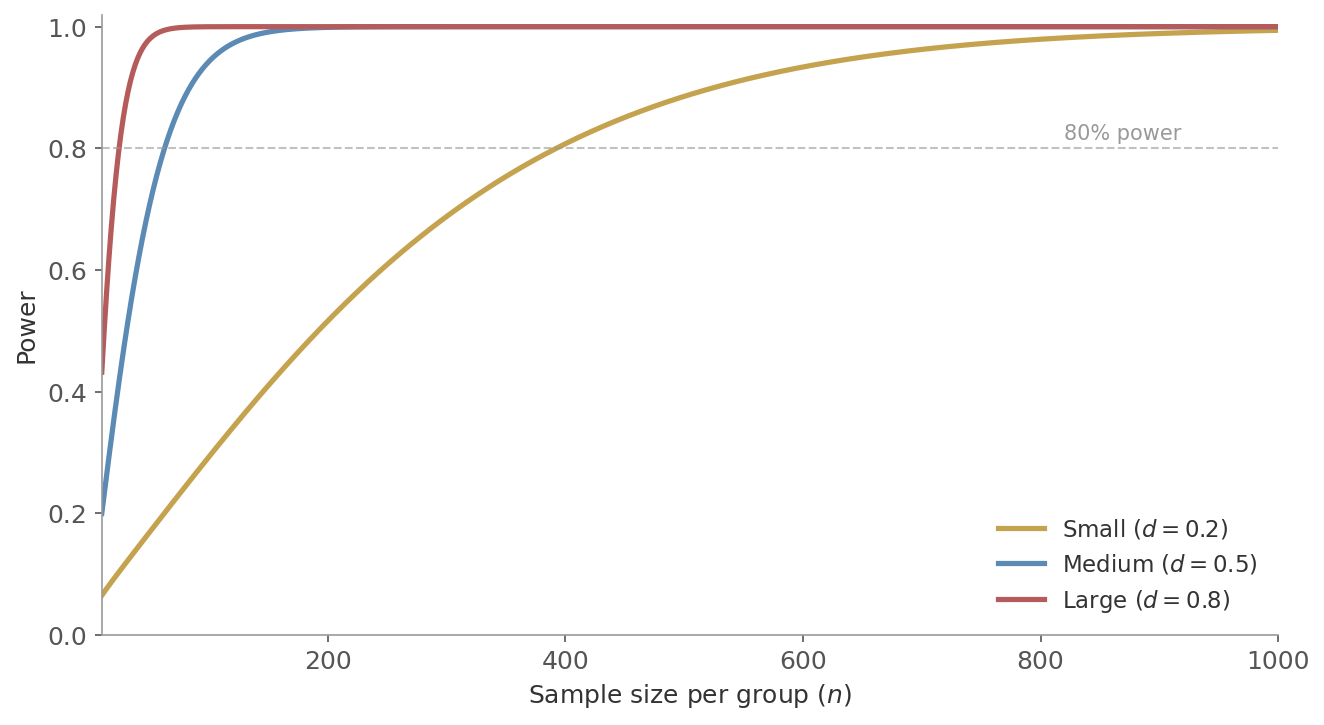$Power vs sample size curves$ Figure 5: Power as a function of sample size per group, for three effect sizes ($\alpha = 0.05$, two-tailed). Large effects ($d = 0.8$) reach 80% power with under 30 per group. Medium effects ($d = 0.5$) need around 65. Small effects ($d = 0.2$) need about 400. The curves flatten as they approach 1.0 - adding more data has diminishing returns once power is already high.

Putting It Together

These concepts form a pipeline. In practice, this is exactly how an A/B test works:

State the hypotheses - what effect are you looking for?
Choose $\alpha$ - how much false positive risk are you willing to accept? (Usually 0.05.)
Choose power - how important is it not to miss a real effect? (Usually 0.80.)
Define the MDE - what’s the smallest effect worth detecting?
Compute sample size - how much data do you need?
Run the experiment and compute the test statistic and p-value.
Decide - reject or fail to reject. Report the confidence interval.

Quick reference

Term	What it means
Significance level $\alpha$	False positive rate - probability of rejecting a true null
$\beta$	False negative rate - probability of missing a real effect
Power	Detection rate - probability of catching a real effect
p-value	How surprising the data is if there’s no effect
Effect size	Standardised magnitude of the difference
Confidence interval	Range of plausible values for the true parameter

Next up: A/B Testing - designing, running, and analysing experiments.