This is part 4 of the ML Fundamentals series.
A decision tree splits data with simple if-then rules. It’s interpretable, handles mixed feature types, and doesn’t need feature scaling. It also overfits badly. Ensemble methods fix that by combining many trees - either in parallel (bagging) or in sequence (boosting). This post covers the full progression: how a single tree works, why it fails, and how combining many trees outperforms any single one.
Decision Trees
A decision tree is a flowchart-like model. Each internal node tests a feature against a threshold. Each branch follows the outcome. Each leaf node holds a prediction - a class label for classification, or a mean value for regression.
The model is built top-down by recursively splitting the data. At each node, the algorithm picks the feature and threshold that best separates the data, then repeats for each child node until a stopping condition is reached.
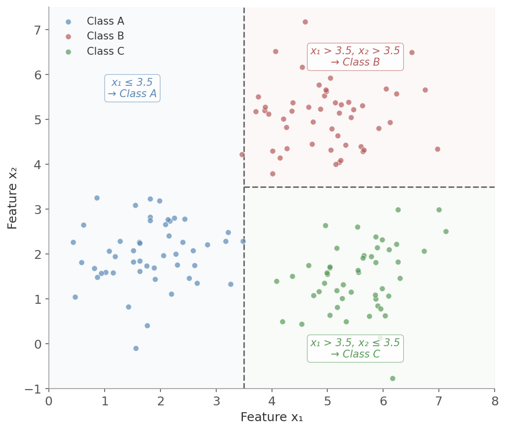 Figure 1: A decision tree partitions feature space with axis-aligned splits. The first split on x₁ = 3.5 separates Class A from the rest. A second split on x₂ = 3.5 separates Class B from Class C. Each colored region corresponds to a leaf node’s prediction.
No feature scaling needed. No assumption of linearity. The tree just carves the space into rectangles with boundaries parallel to the feature axes.
Splitting Criteria
The key question at each node: which feature and threshold produce the best split? “Best” means the resulting child nodes are as pure as possible - ideally containing only one class.
Three impurity measures are used in practice.
where $p_i$ is the proportion of class $i$ at node $t$. Entropy measures uncertainty: 0 when a node is pure (all one class), maximum when classes are evenly mixed.
Entropy comes from information theory. A node where 100% of examples belong to one class has zero entropy - no uncertainty about the label. A 50/50 split has entropy of 1 bit - maximum uncertainty for binary classification.
The entropy before the split minus the weighted average entropy after the split. The weights are the proportion of examples going to each child. Higher information gain means the split removed more uncertainty.
Say we have a dataset $S$ of 10 people:
- 6 bought a product (positive)
- 4 did not (negative)
Step 1: Compute entropy of the whole set
$$H(S) = -\left(\frac{6}{10}\log_2\frac{6}{10} + \frac{4}{10}\log_2\frac{4}{10}\right) \approx 0.97$$Step 2: Suppose we split by “Age > 30”
- Left branch: 5 examples - 4 positive, 1 negative - entropy $\approx 0.72$
- Right branch: 5 examples - 2 positive, 3 negative - entropy $\approx 0.97$
Step 3: Weighted entropy after split
$$= \frac{5}{10} \cdot 0.72 + \frac{5}{10} \cdot 0.97 = 0.845$$Step 4: Information gain
$$IG = 0.97 - 0.845 = 0.125$$The feature “Age > 30” reduced uncertainty by 0.125 bits - it helps, but maybe there’s a better feature to split on.
The tree greedily picks the split that maximizes information gain at each step. “Greedy” means it doesn’t look ahead - it picks the locally best split without considering what future splits might be possible.
The probability that a randomly chosen example from node $t$ would be misclassified if labeled according to the class distribution at that node. Like entropy, it’s 0 for a pure node and maximal for an even split.
Case 1: All examples are class 1 (pure)
$p_1 = 1, \quad p_2 = 0$
$$G = 1 - (1^2 + 0^2) = 0$$Case 2: Half class 1, half class 2 (most impure)
$p_1 = 0.5, \quad p_2 = 0.5$
$$G = 1 - (0.5^2 + 0.5^2) = 1 - 0.5 = 0.5$$Case 3: 80% class 1, 20% class 2
$p_1 = 0.8, \quad p_2 = 0.2$
$$G = 1 - (0.64 + 0.04) = 1 - 0.68 = 0.32$$To evaluate a split, compute the weighted Gini of the child nodes and subtract from the parent’s Gini - the same idea as information gain, just using Gini instead of entropy.
Classification error ($1 - \max(p_i)$) is a third option but is less commonly used. It’s not as sensitive to changes in class probabilities near the even-split region, which makes it worse at finding good splits. It’s occasionally used for pruning, not for growing trees.
Using the same three cases:
- Pure node ($p_1 = 1.0$): $E = 1 - 1.0 = 0$
- 50/50 split ($p_1 = 0.5$): $E = 1 - 0.5 = 0.5$
- 80/20 split ($p_1 = 0.8$): $E = 1 - 0.8 = 0.2$
Compare with Gini for the 80/20 case: classification error gives 0.2, Gini gives 0.32. The classification error is less sensitive to changes near the pure end - it doesn’t penalize a 70/30 split much more than an 80/20 split. Gini and entropy both react more strongly to these differences, which is why they’re better for growing trees.
| Criterion | Formula | Measures | Sensitivity |
|---|---|---|---|
| Entropy | $-\sum p_i \log_2 p_i$ | Information content | High |
| Gini Impurity | $1 - \sum p_i^2$ | Misclassification probability | Medium |
| Classification Error | $1 - \max(p_i)$ | Misclassification rate | Low |
Sensitivity here means how strongly a criterion reacts to changes in class probabilities - especially near the even-split region where the decision matters most. For a 90/10 node:
- Entropy: $H \approx 0.47$ - reacts sharply to even slight mixing, strong preference for pure splits
- Gini: $G = 1 - (0.81 + 0.01) = 0.18$ - less steep but still penalizes impurity well, faster to compute (no logarithm)
- Classification error: $E = 1 - 0.9 = 0.1$ - only cares about the majority class, ignores how mixed the rest are
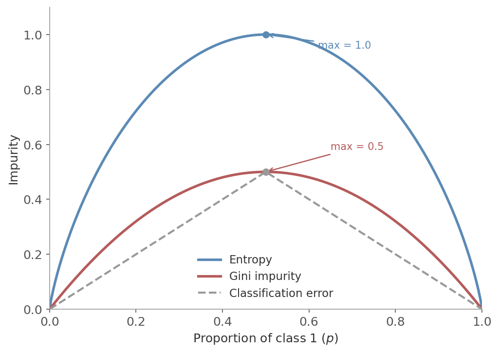 Figure 2: Impurity as a function of the class 1 proportion $p$ in a binary classification node. Entropy (blue) peaks at 1.0 when $p = 0.5$, Gini impurity (red) peaks at 0.5. Both curves are concave and reach zero at the extremes (pure nodes). The dashed line is classification error - flatter near $p = 0.5$, so less sensitive to improvements in that region.
Both produce nearly identical trees most of the time. Gini is slightly faster to compute (no logarithm). Scikit-learn uses Gini by default. Unless you have a specific reason to prefer one, the choice rarely matters.
For regression trees, the splitting criterion is different. Instead of impurity, the algorithm minimizes the variance (or equivalently, MSE) within each child node. Each leaf predicts the mean of the target values that land in it.
Overfitting
An unrestricted decision tree will keep splitting until every leaf is pure - one example per leaf. This memorizes the training data perfectly and generalizes terribly. The tree learns noise, not patterns.
Common controls:
- Max depth: limit how many levels deep the tree can grow
- Min samples per leaf: require a minimum number of examples in each leaf
- Min samples per split: require a minimum number of examples in a node before it can be split
- Pruning: grow the full tree first, then remove branches that don’t improve validation performance. This can find a better structure than pre-pruning because it considers the full tree before cutting
Even with these controls, single trees are unstable - small changes in the training data can produce very different trees. This is where ensembles come in.
Ensemble Methods
The idea is simple: combine multiple models to get a better result than any single one could achieve.
Two main strategies:
- Bagging: train models independently in parallel on different subsets of data. Reduces variance
- Boosting: train models sequentially, where each model focuses on the errors of the previous one. Reduces bias
Both approaches work well with decision trees as the base learner.
Bagging
Bootstrap Aggregating (bagging) works as follows:
- Draw $B$ bootstrap samples from the training data (sample with replacement, same size as original)
- Train one model (typically a decision tree) on each bootstrap sample
- Aggregate predictions: majority vote for classification, average for regression
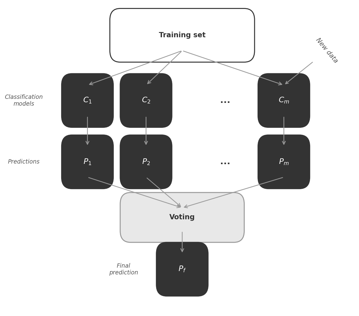 Figure 3: Bagging trains multiple classifiers ($C_1, C_2, \ldots, C_m$) independently on bootstrap samples, each producing its own prediction. The final prediction $P_f$ is determined by majority vote (classification) or averaging (regression).
Why Bagging Reduces Variance
If you average $B$ independent predictions each with variance $\sigma^2$, the variance of the average is:
$$\text{Var}\left(\frac{1}{B}\sum_{b=1}^{B} X_b\right) = \frac{\sigma^2}{B}$$Averaging $B$ independent predictions reduces variance by a factor of $B$. Bagging applies this idea to models: train each one on a different bootstrap sample and average the predictions.
In practice, bagged trees aren’t truly independent - they train on overlapping data and may split on the same dominant features. The actual variance of the average depends on the pairwise correlation $\rho$ between trees:
$$\text{Var} = \rho\sigma^2 + \frac{1-\rho}{B}\sigma^2$$When $\rho = 0$ (independent trees), this reduces to $\sigma^2/B$. When $\rho = 1$ (identical trees), averaging does nothing. The key is keeping $\rho$ low - which is exactly what random forests address.
Bagging still works well because bootstrap sampling creates enough diversity that errors partially cancel. And it pairs particularly well with decision trees - trees are inherently high-variance, so small changes in training data produce very different splits. That instability is a liability for a single tree, but it’s exactly what bagging needs: diverse models whose errors don’t all point in the same direction.
Random Forests
Random forests are the main bagging method in practice. They add a second source of randomness on top of bootstrap sampling: at each split, only a random subset of features is considered.
The algorithm:
- Draw a bootstrap sample of size $n$ (with replacement) from the training data
- Grow a decision tree from this sample. At each node:
- Randomly select $d$ out of the total $p$ features (without replacement)
- Find the best split among only those $d$ features
- Repeat steps 1-2 for $B$ trees
- Aggregate: majority vote (classification) or average (regression)
The two sources of randomness - bootstrap samples and random feature subsets - ensure that the individual trees are diverse. Without the feature randomization, if one feature is strongly predictive, every tree would split on it first and the trees would be highly correlated. Correlated models don’t benefit much from averaging.
Key hyperparameters:
| Parameter | Description | Typical default |
|---|---|---|
n_estimators | Number of trees | 100-500 |
max_features | Features considered per split | $\sqrt{p}$ (classification), $p/3$ (regression) |
max_depth | Maximum tree depth | None (fully grown) |
min_samples_leaf | Minimum examples per leaf | 1 |
max_samples | Bootstrap sample size | $n$ (same as training set) |
More trees almost always help (or at least don’t hurt) - unlike boosting, random forests are relatively robust to using too many trees. The main cost is computation time.
The two most impactful tuning knobs beyond tree count:
max_features ($d$) - features considered at each split:
- Fewer features → more tree diversity, less overfitting, but weaker individual trees
- More features → stronger individual trees, but more correlated (and correlated trees don’t benefit from averaging)
- Defaults ($\sqrt{p}$ for classification, $p/3$ for regression) balance this well
max_samples ($n$) - bootstrap sample size:
- Typically set equal to the training set size
- Smaller samples → more diversity (trees are less correlated), but lower individual tree quality
- Larger samples → risk overfitting as each tree sees more of the original data
Feature importance: random forests rank features by the total impurity decrease they provide, averaged across all trees. A feature that appears in many splits and produces large impurity reductions is considered important.
Impurity-based feature importance has known biases:
- High-cardinality features (many unique values, like IDs or zip codes) get inflated importance because they offer more possible split points
- Correlated features share importance unpredictably - one might rank high while an equally informative correlated feature ranks low
For more reliable feature attribution, use permutation importance or SHAP values - covered in the regularization post.
Out-of-bag (OOB) score: each bootstrap sample leaves out about 37% of the training data (the probability of not being selected in $n$ draws with replacement is $(1-1/n)^n \approx 1/e$). These left-out examples provide a free validation set. The OOB score evaluates each example using only the trees that didn’t see it during training, giving an honest estimate of generalization error without needing a separate validation set.
Boosting
Bagging trains models in parallel and averages them. Boosting trains models sequentially - each new model focuses on the mistakes of the previous ones.
Gradient boosting builds a series of shallow trees where each tree fits the pseudo-residuals of the previous ensemble. Each round nudges the predictions closer to the correct answer via small updates in the direction of the loss gradient - which is how gradient boosting got its name.
 Figure 4: The boosting process. Each round trains a new model that focuses on examples the previous ensemble got wrong. The individual models combine into a final prediction that’s stronger than any single one.
The algorithm:
- Initialize with a constant prediction: $F_0(x) = \arg\min_c \sum_{i=1}^{n} L(y_i, c)$
- For each iteration $t = 1$ to $T$:
- Compute pseudo-residuals: $r_i = -\frac{\partial L(y_i, F_{t-1}(x_i))}{\partial F_{t-1}(x_i)}$ (the negative gradient of the loss)
- Fit a decision tree $h_t$ to the pseudo-residuals
- Update the model: $F_t(x) = F_{t-1}(x) + \nu \cdot h_t(x)$ where $\nu$ is the learning rate
- Final model: $F_T(x) = F_0(x) + \nu \sum_{t=1}^{T} h_t(x)$
The term “pseudo-residuals” is important. For MSE loss, the pseudo-residuals are just the ordinary residuals $(y_i - \hat{y}_i)$. But gradient boosting works for any differentiable loss function. For log-loss (classification), the pseudo-residuals point in the direction that most reduces the log-loss. This is what makes gradient boosting so flexible - it reduces to gradient descent in function space.
Key hyperparameters:
| Parameter | Description | Typical range |
|---|---|---|
n_estimators | Number of boosting rounds | 100-1000+ |
learning_rate | Step size per iteration ($\nu$) | 0.01-0.3 |
max_depth | Depth of each tree | 3-8 (shallow) |
subsample | Fraction of data per tree | 0.5-1.0 |
The learning rate and number of estimators are tightly coupled: a smaller learning rate needs more trees but generalizes better. The standard approach is to set a low learning rate (0.05-0.1) and use early stopping to find the right number of trees.
Early stopping: instead of picking n_estimators upfront, train until validation performance stops improving. At each round, evaluate the ensemble on a held-out validation set. When the validation loss hasn’t decreased for a set number of rounds (the “patience” parameter), stop training. This prevents overfitting and removes the need to tune the number of trees manually - the model decides for itself.
Stochastic gradient boosting: setting subsample < 1.0 fits each tree to a random fraction of the training data. This adds noise that acts as regularization - similar in spirit to the bootstrap sampling in bagging - and often improves generalization while also speeding up training.
These are optimized implementations of gradient boosting, not fundamentally different algorithms. In practice, any of the three is a strong default choice for tabular data.
- XGBoost: adds L1/L2 regularization terms to the objective function (penalizing tree complexity directly, not just prediction error) and handles sparse data efficiently by learning default split directions for missing values
- LightGBM: buckets continuous features into discrete histogram bins to speed up split finding (fewer thresholds to evaluate), and grows trees leaf-wise (always splitting the leaf with the highest loss reduction) rather than level-by-level - faster convergence but can overfit on small datasets
- CatBoost: handles categorical features natively using ordered target encoding (avoids the need for manual one-hot or label encoding), and uses ordered boosting to reduce prediction shift (a subtle form of target leakage in standard gradient boosting)
Bagging vs Boosting
| Bagging (Random Forest) | Boosting (Gradient Boosting) | |
|---|---|---|
| Training | Parallel (independent models) | Sequential (each depends on previous) |
| Data sampling | Bootstrap samples (with replacement) | Full dataset, fits to residuals each round |
| Reduces | Variance | Bias |
| Base learners | Deep trees (high variance) | Shallow trees (high bias) |
| Overfitting risk | Low - more trees rarely hurts | Higher - can overfit if not tuned |
| Key tuning | n_estimators, max_features | learning_rate, n_estimators, max_depth |
| Speed | Parallelizable | Sequential (slower per tree count) |
Bagging takes high-variance models and stabilizes them through averaging. Boosting takes high-bias models and progressively corrects their systematic errors. Both improve over a single tree, but they attack different problems.
Practical Notes
Decision trees are the right choice when interpretability is the priority. A single tree can be visualized and explained to non-technical stakeholders. Use them for exploratory analysis or when model transparency is a requirement.
Random forests are the reliable workhorse. They work well out of the box with minimal tuning, handle missing values and mixed feature types, and rarely overfit catastrophically. A random forest is often the first model worth trying on a new tabular dataset.
Gradient boosting typically achieves the best performance on tabular data - but requires more careful tuning. The learning rate, tree depth, and number of iterations all interact. Without early stopping and proper cross-validation, it can overfit. The payoff is often a few percentage points of performance over random forests.
| Decision Tree | Random Forest (Bagging) | Gradient Boosting | |
|---|---|---|---|
| Pros | Interpretable, no feature scaling, handles mixed types | Robust to overfitting, feature importance, noise-resistant, no scaling, minimal tuning | Best performance on tabular data, flexible loss functions, handles complex patterns |
| Cons | Overfits easily, unstable (small data changes → different tree) | Loses interpretability, higher memory/compute, slower than single tree | Requires careful tuning, can overfit, sequential (not parallelizable), slower to train |
| Reduces | - | Variance | Bias |
| Key tuning | max_depth, min_samples_leaf | n_estimators, max_features | learning_rate, n_estimators, max_depth |
| When to use | Interpretability, exploration | Strong baseline, quick results | Max performance with tuning budget |
Next in the ML Fundamentals series: logistic regression - from predicting values to classifying categories.